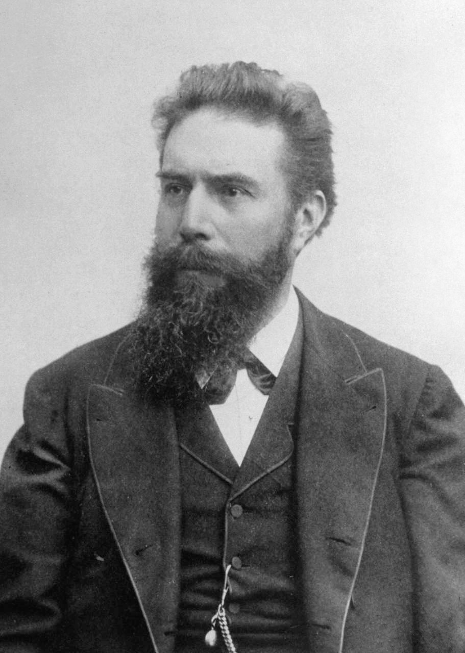
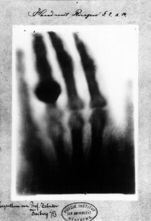
Wilhem Röntgen a German physicist made the discovery in 1895 of X-rays during
studies of vacuum tubes (Crookes). The first x-rays on film (the
hand of his wife) date from this period.
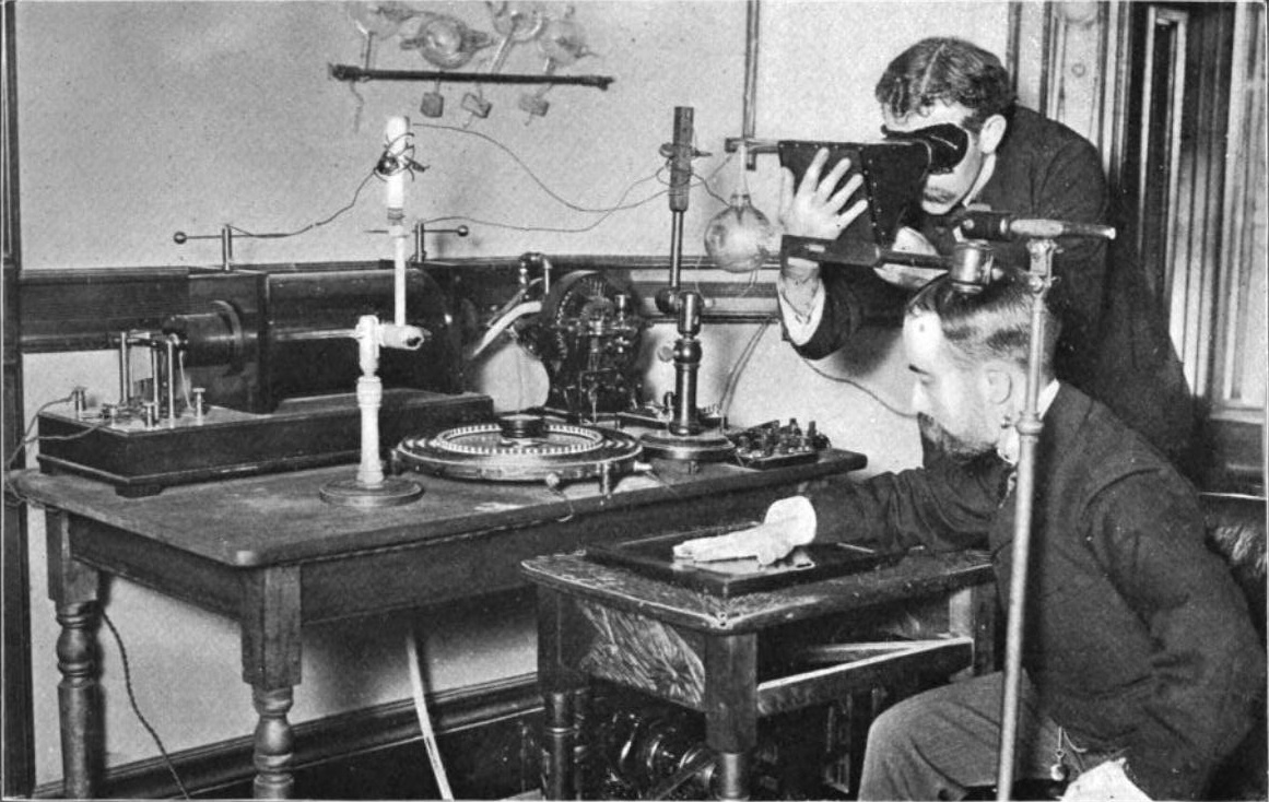
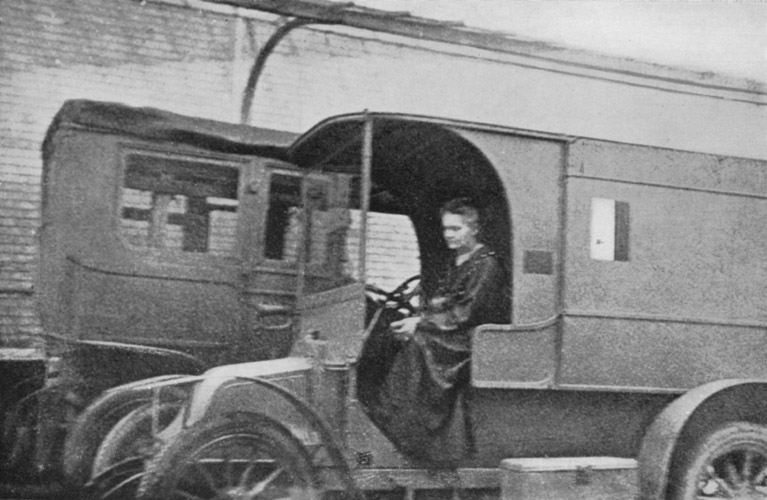
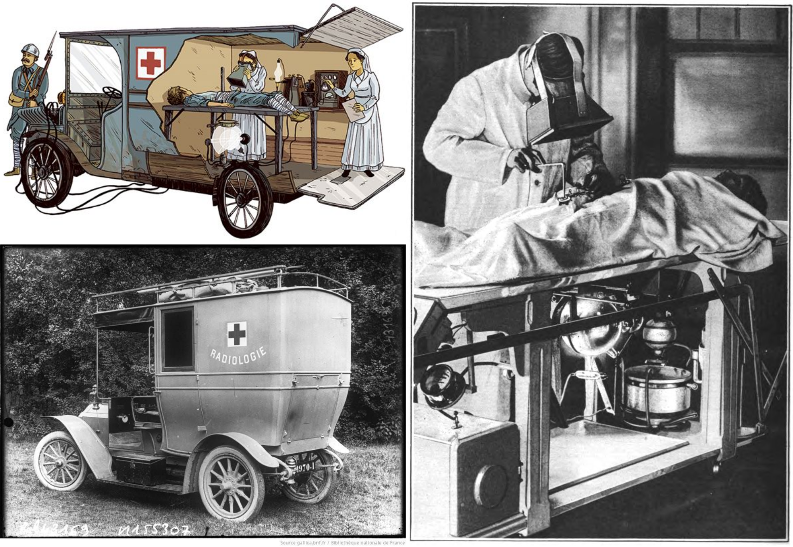
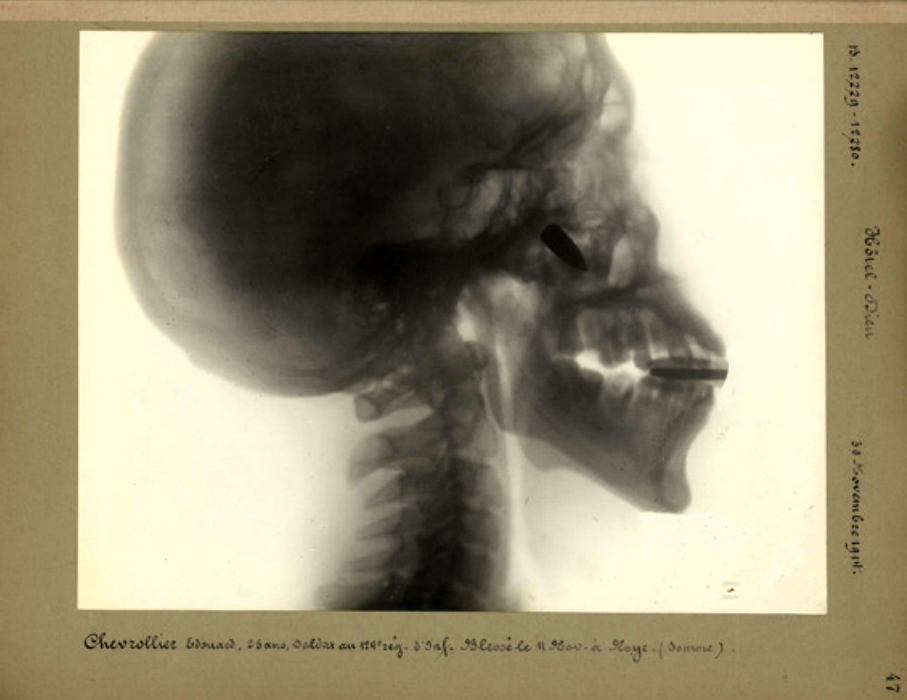
Less than 20 years after their discovery, X-ray imaging was used medicinally in battle fields.
Marie Curie, Nobel Prize winner in physics and chemistry, participates in the design of mobile radiology surgical units (see Petites Curies).
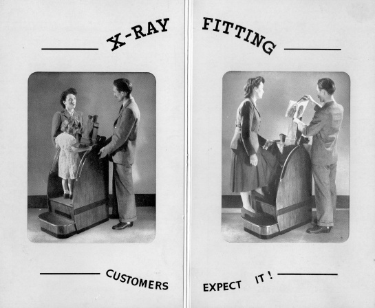
Some societal applications of X-rays appeared in the first half of the 20th century
century, but radiobiological studies quickly put an end to these applications.
X-rays can be modeled twofold (it is the wave-particle duality):
as massless particles called photons characterised by their energy usually expressed in keV.
The keV unit is used instead of Joules by reference to the mode of x-ray production which is
based on electron acceleration: the kinetic energy of an electron (initially at rest)
accelerated by a potential difference of 1V is 1eV. The speed of light in vaccum is \(3\times 10^8\) m\(\cdot\)s\(^{-1}\).
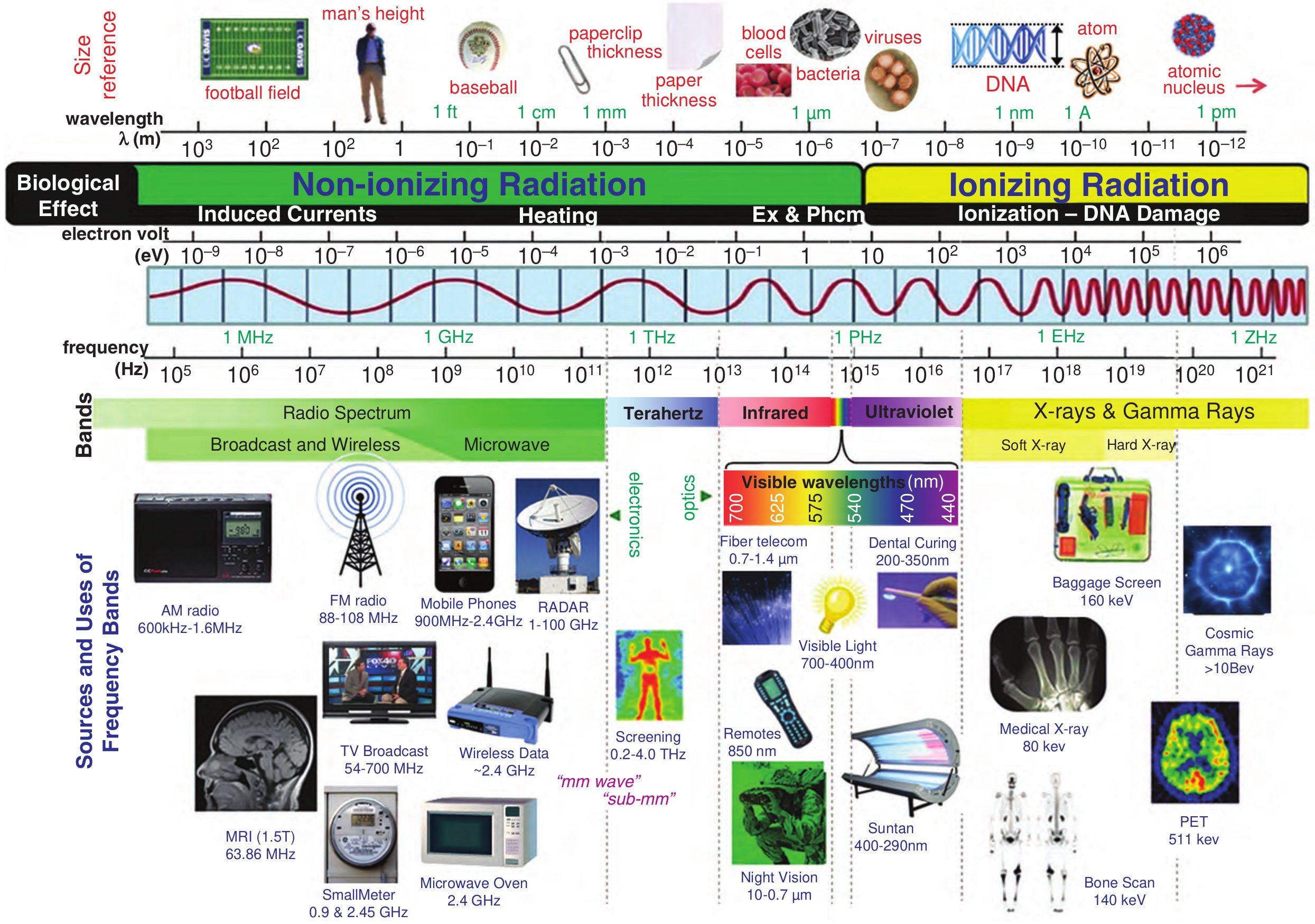
or else as electromagnetic radiation, characterized by its wavelength. The range of electromagnetic radiation is very wide.
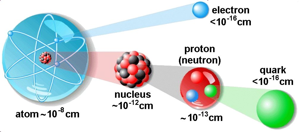
The wavelength of x-rays is less than nm: atoms and their constituents are
therefore resolved.
Photon
The photon energy \(E\) is related to the photon frequency \(\nu\):
\[
E = h\nu
\]
When all photons of an x-ray beam have the same energy, the x-ray beam is called “monochromatic”, and named “polychromatic” otherwise. The momentum \(\mathbf{p}\) and wave vector \(\mathbf{k}\) are given by:
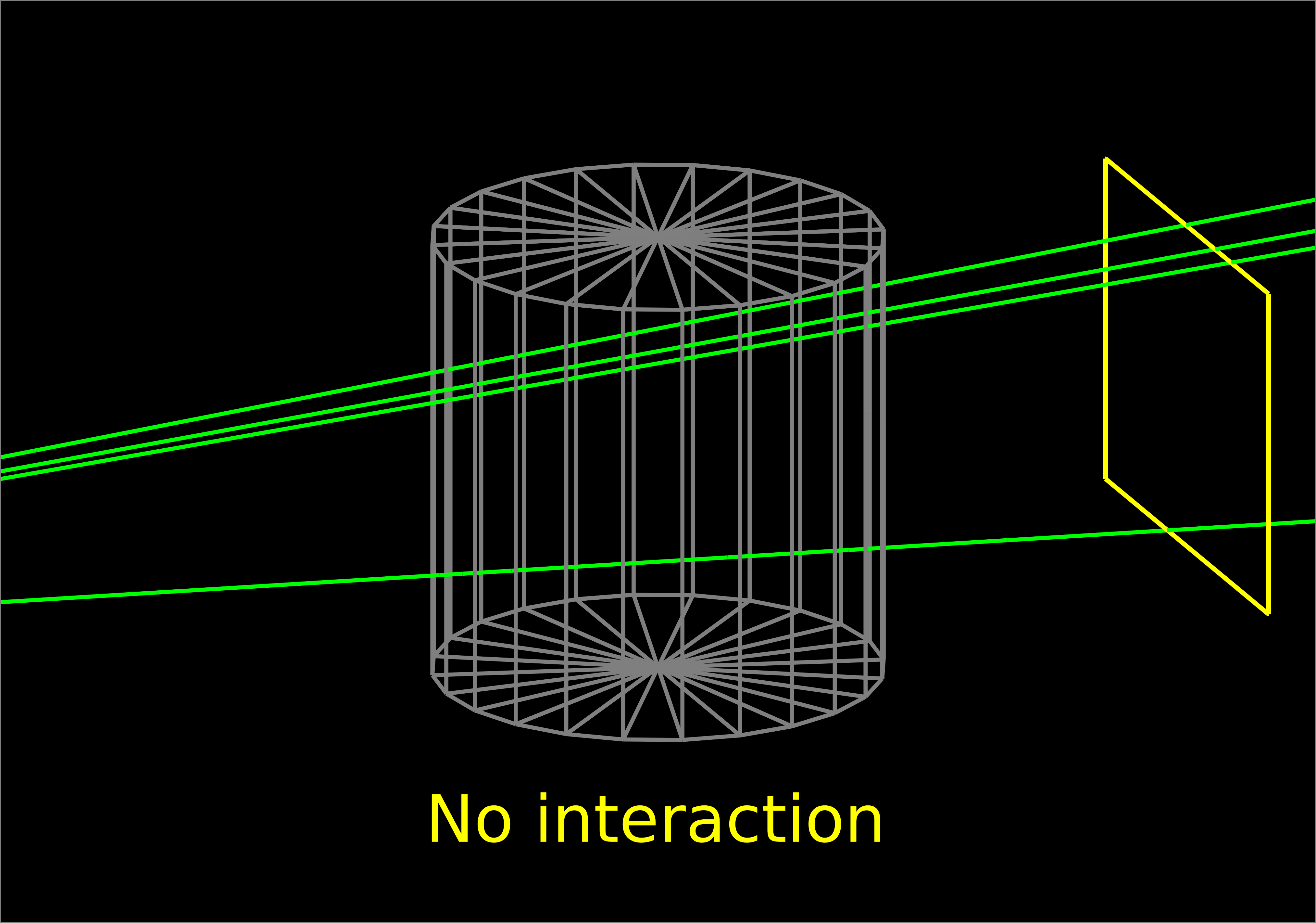
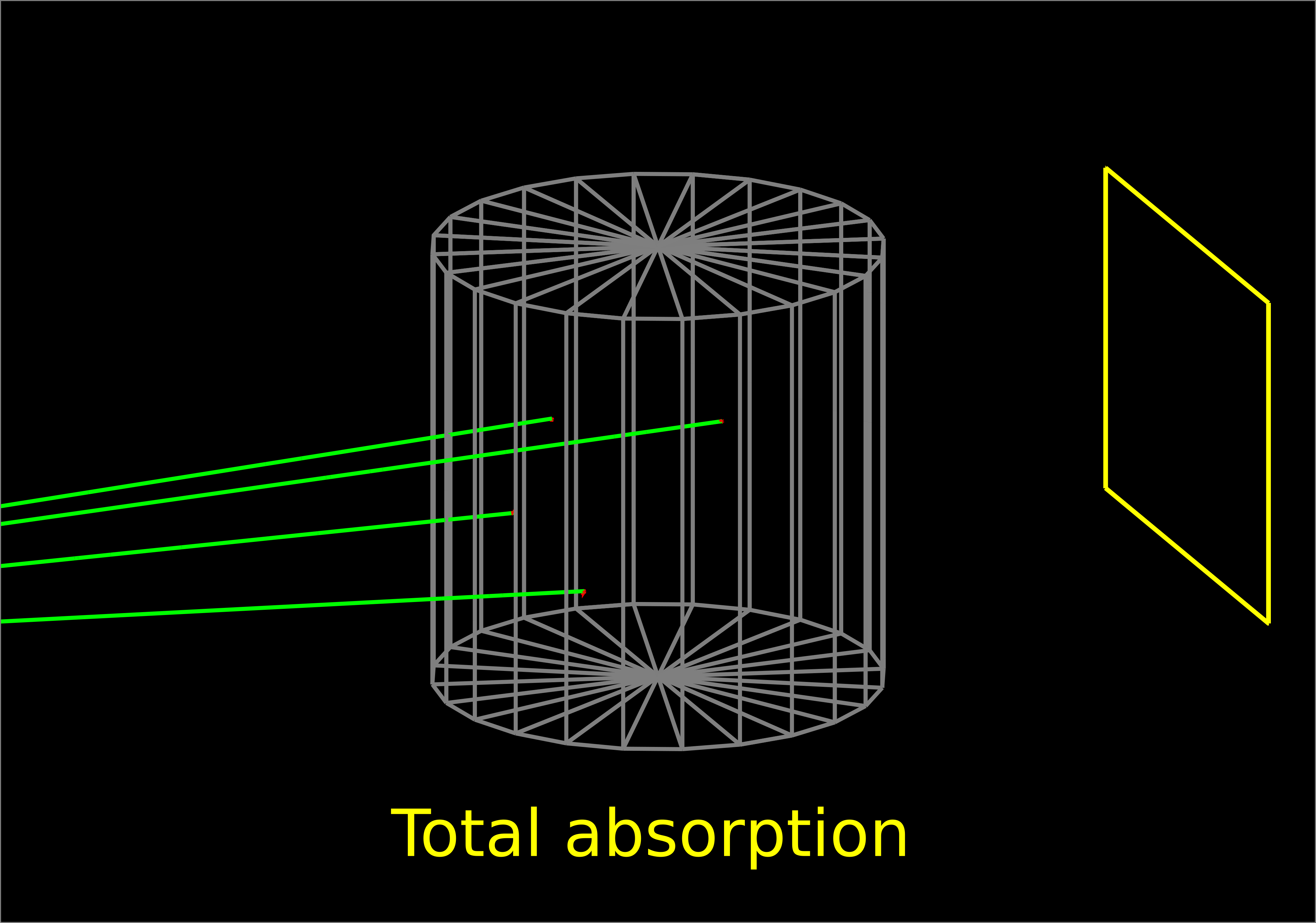
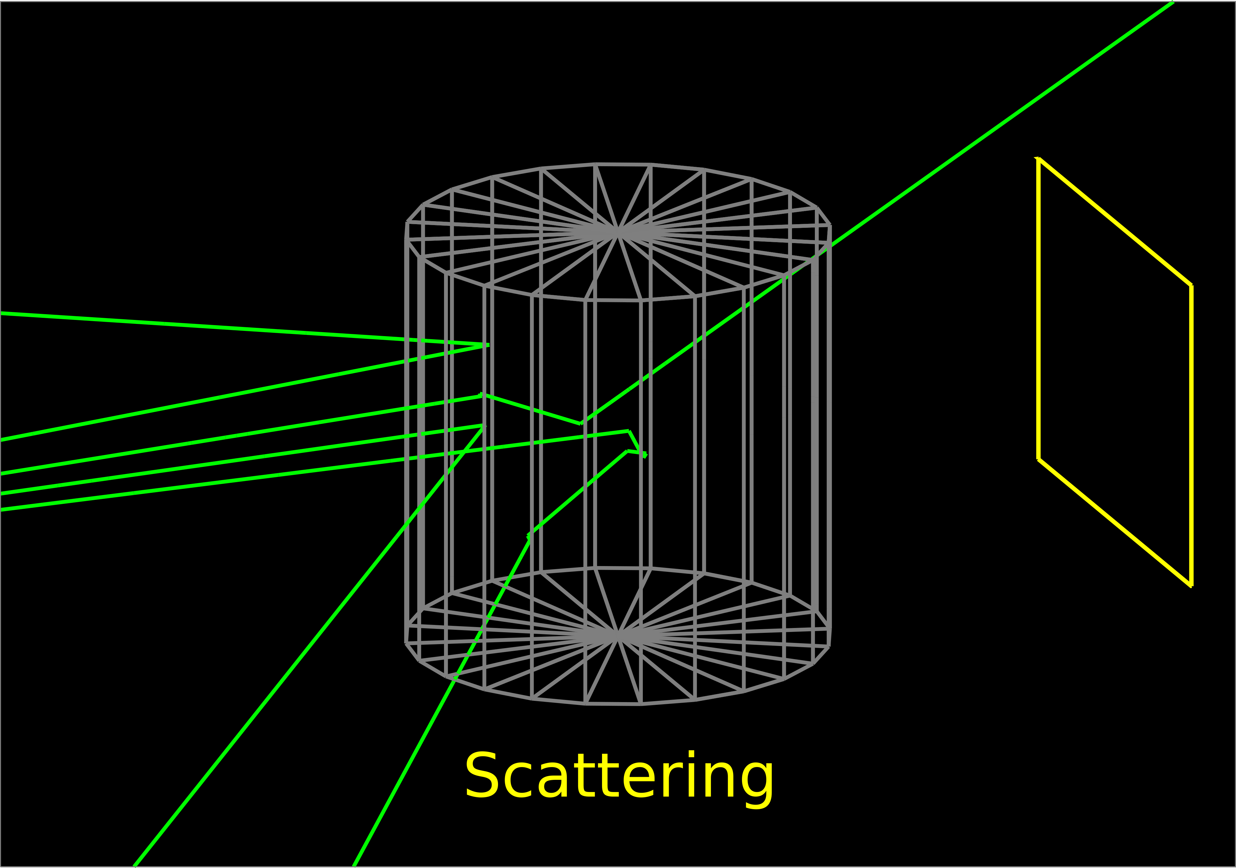
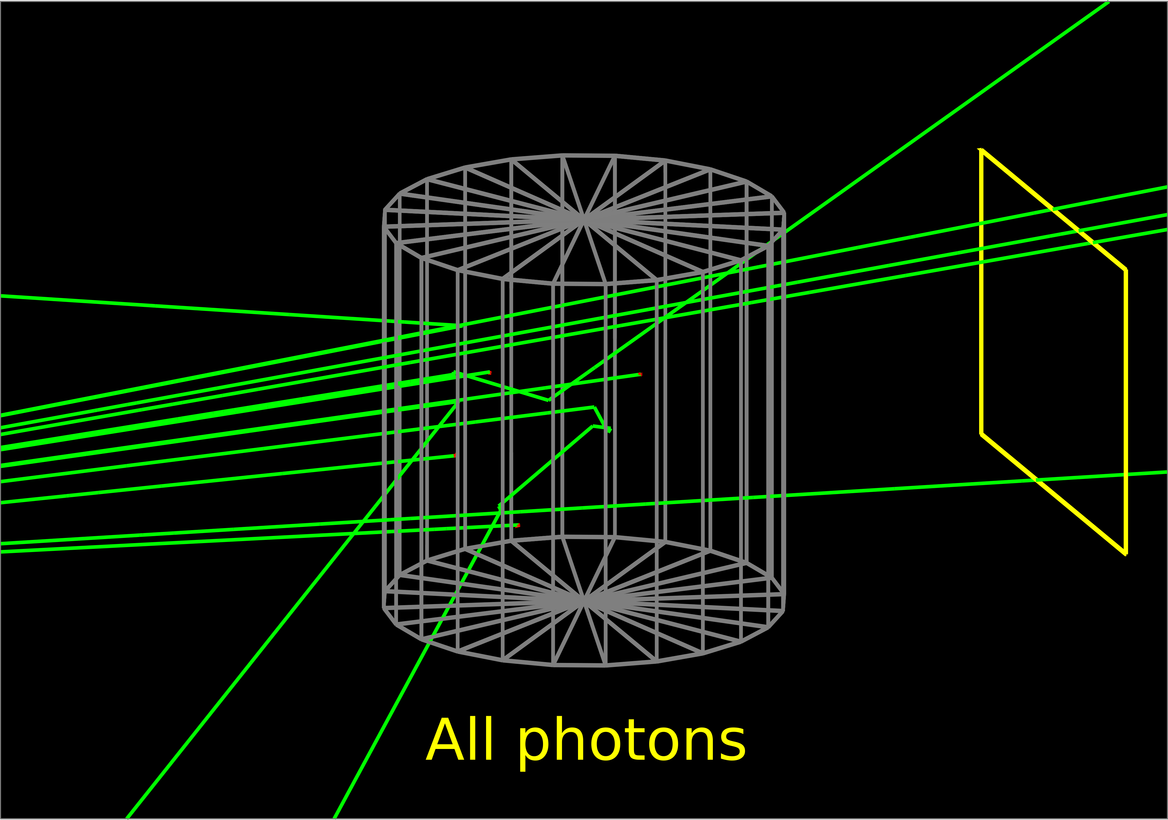
Photon-matter interactions are of two types: total absorption or scattering. In
in the first case the energy of the photon is locally transferred to the atom. In the second
case, a scattered photon is emitted after interaction with its own energy and direction.
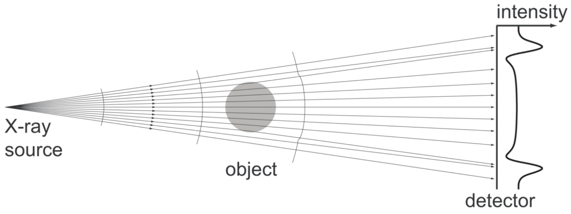
X-ray imaging is therefore based on attenuation, ie the proportion of photons that does not have
any interaction with the matter, namely the radiation directly transmitted. This is the Beer-Lambert law.
Fig. 24 Interactions of photons with matter: direct transmission + total absorption + scattering#
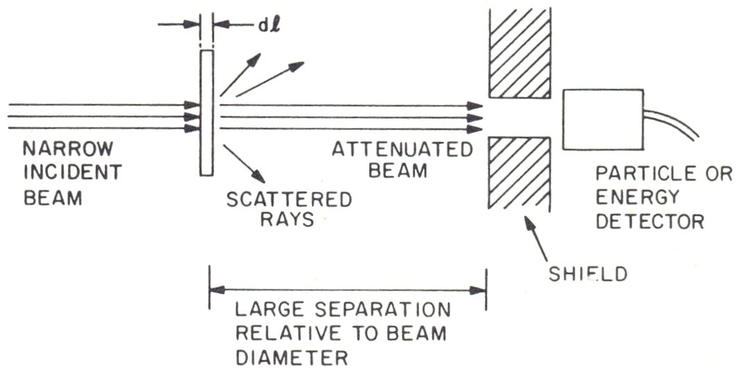
Beer-Lambert attenation law: ratio of photons
\[
\frac{\mbox{Number of photons transmitted with no interaction}}{\mbox{Number of emitted photons}}
\]
The law of attenuation can be deduced from a thin beam model impinging on a plate of elementary thickness \(\text{d}l\). The drop in the number of directly transmitted photons is proportional to the number of incident photons \(N\) and the thickness of this plate.
\(\mu\) is therefore a linear attenuation coefficient which corresponds to a percentage of interaction per unit length.
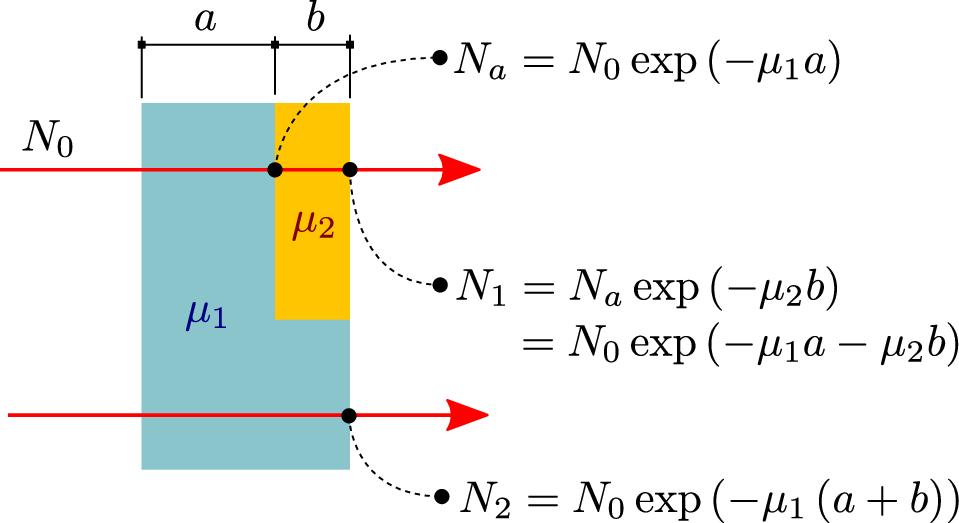
Integrating this equation gives the exponential law of attenuation which presents a
simple shape in the case of a homogeneous material and for a single radiation
energy \(E\).
In the case of materials with several homogeneous phases, the attenuation results from simple
product of attenuations on the different constituent materials. In fact, for a locally non-divergent
geometry, the order and positioning of the materials long radiation has no influence on the number
of photons directly transmitted (unlike the proportion of scattered radiation arriving on the
detector).
The Beer-Lambert law of attenuation generalizes to spectra large and heterogeneous materials in the
form of a sum of exponentials. She can be expressed in number of photons, in energy, or in dose.
Generalized Beer-Lambert law for a polychromatic // beam and an heterogeneous material
The linear attenuation coefficient \(\mu\), which is the probabibility of interation per unit length, can be therefore interpreted as the sum over the different x-ray interactions with matter.
Linear attenuation coefficient \(\mu\)
The linear attenuation coefficient \(\mu\) is a sum of interaction probabilities per unit length (i.e. in cm\(^{-1}\))
The linear attenuation coefficient \(\mu\) varies linearly with the material density \(\rho\) and the cross
section \(\sigma\), which represents a probability of interaction expressed as an area.
The cross-section \(\sigma\) does not depend on the material density \(\rho\). The mass attenuation coefficient \({\mu}/{\rho}\), which is expressed in \(\text{cm}^2\cdot\text{g}^{-1}\), is therefore independent of the density \(\rho\)
The Bragg additivity rule makes it possible to relate the mass attenuation coefficient \({\mu}/{\rho}\)
to calculate that of a mixture.
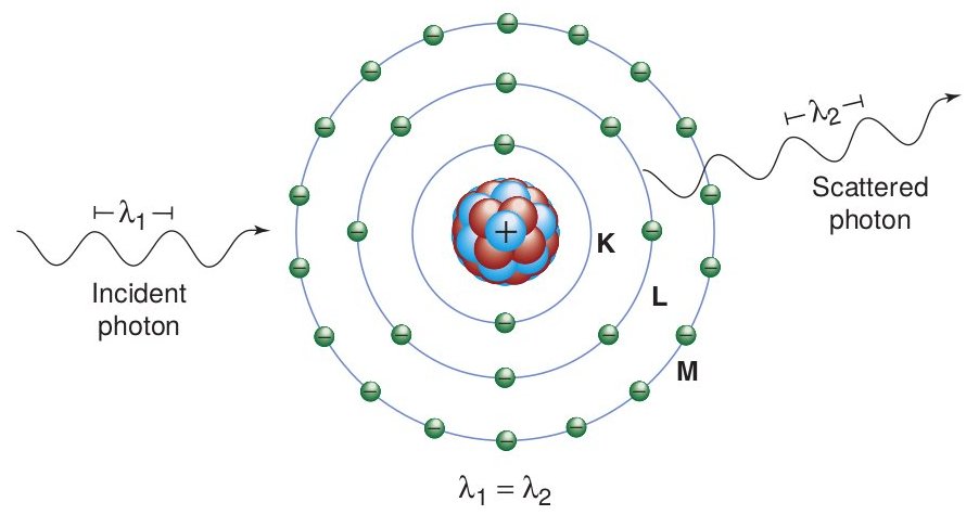
total cross section \({\sigma_R}\left/{\rho}\right. \propto Z\left/E^2\right.\)
small scattering angle
no excitation/ionization
atom recoil-energy negligible \(E_{\mathrm{scatter}} = E\)
The scattered photon has a differential (angular) cross section, denoted DCS, maximum in the
incident direction, ie the angle of scattering \(\theta \approx 0\).
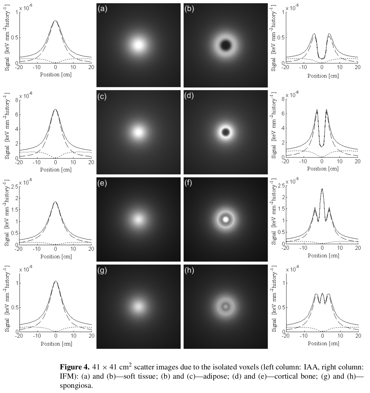
The interest of this scattering is its sensitivity to atomic arrangement. For materials different
but having the same attenuation, Rayleigh broadcast DCS can be very different. The independent atom
approximation (IAA) is not good enough for modelling scattering compared to a more complex
interference function model (IFM) to take into account extra-atomic interference (see Fig. 30 where the Rayleigh DCS is plotted in long-dashed lines).
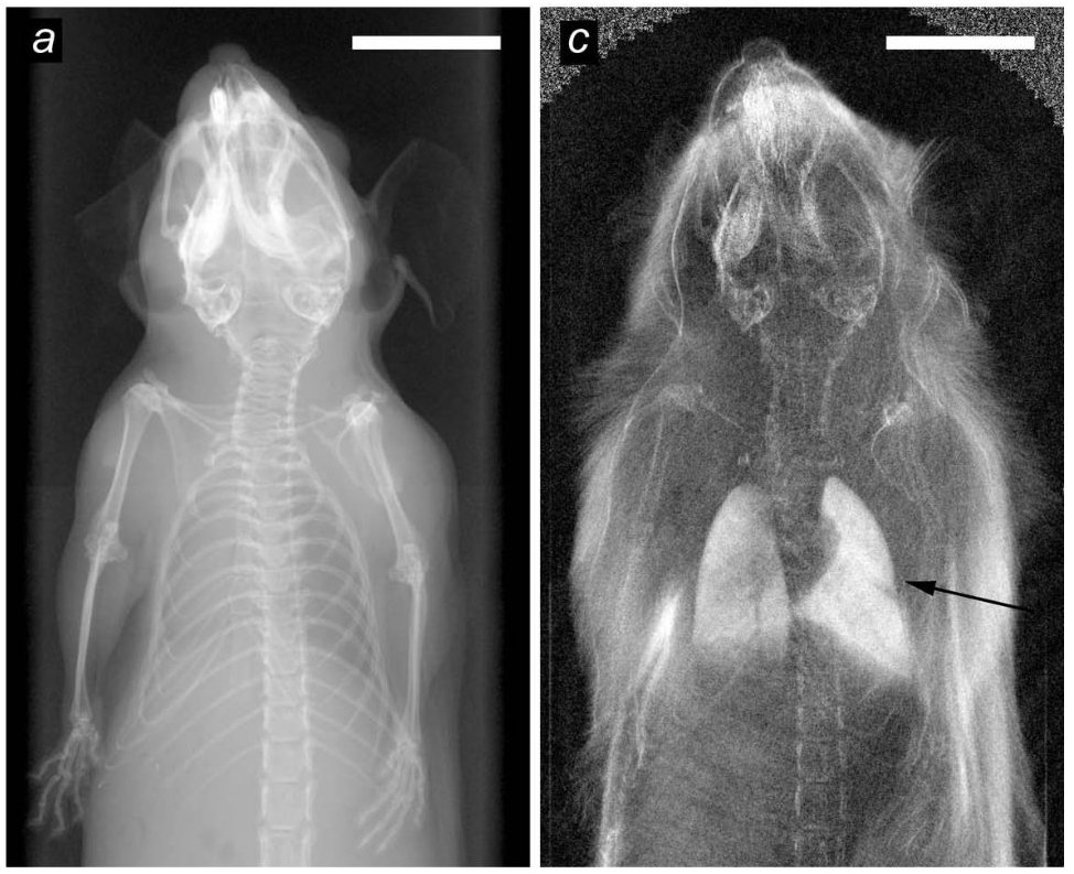
It is the idea of so-called dark field imagery that allows puts access
to these DCS by Talbot-Lau interferometry. The information thus extracted are complementary to those
of simple attenuation.
Fig. 31 From Bech Nature Sci Rep 2013 DOI. Both images acquired with a \(31\;\text{kV}\) beam: (a) Conventional x-ray image based on attenuation, (c) Dark-field image based on Rayleigh scattering (using a Talbot-Lau x-ray interferometer)#
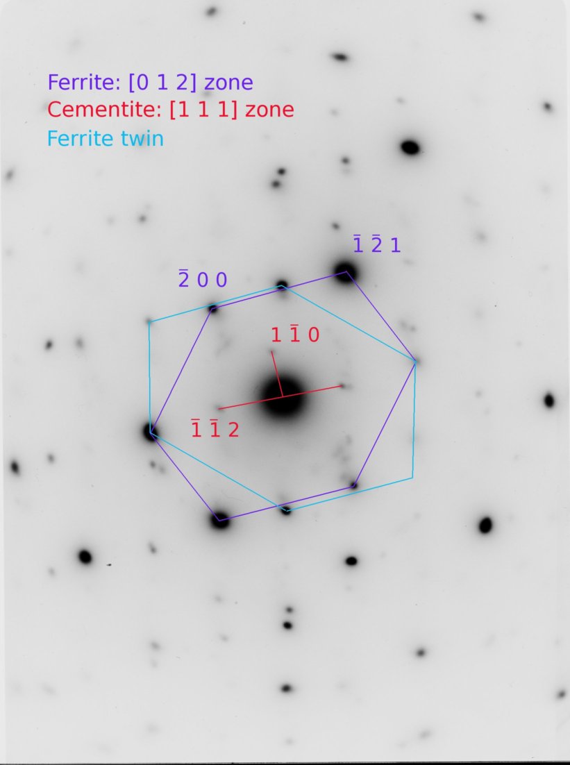
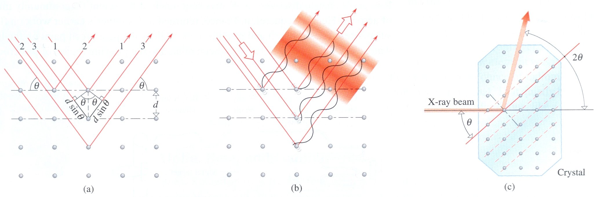
Regular atomic arrangements generate diffraction patterns in directions related to Bragg’s law
according to the directions of the planes of atoms. This gives rise to small (SAXS) or wide angle
(WAXS) diffraction imaging techniques.
Fig. 32 Diffraction patterns. Two ferrite crystals in twin orientation and one cementite precipitate. Data from Lucy Fielding.#
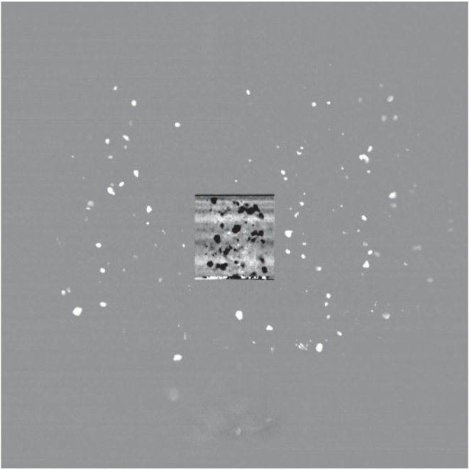
Fig. 34 Radiography for DCT showing both transmitted and diffracted images. From Rolland du Roscoat AEM 2010 DOI#
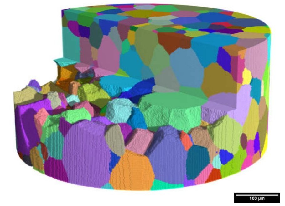
Fig. 35 DCT reconstruction of a sample of Ti alloy Tib21s. From King NIMB 2010 DOI#
Teams recently proposed a diffraction contrasy tomography (DCT) combining
attenuation and diffraction on the same detector. Diffraction spots are associated in pairs at \(\pi\)
angular distance during the rotation of the source, which makes it possible to find the local
orientation of the atomic structure (see Fig. 35).
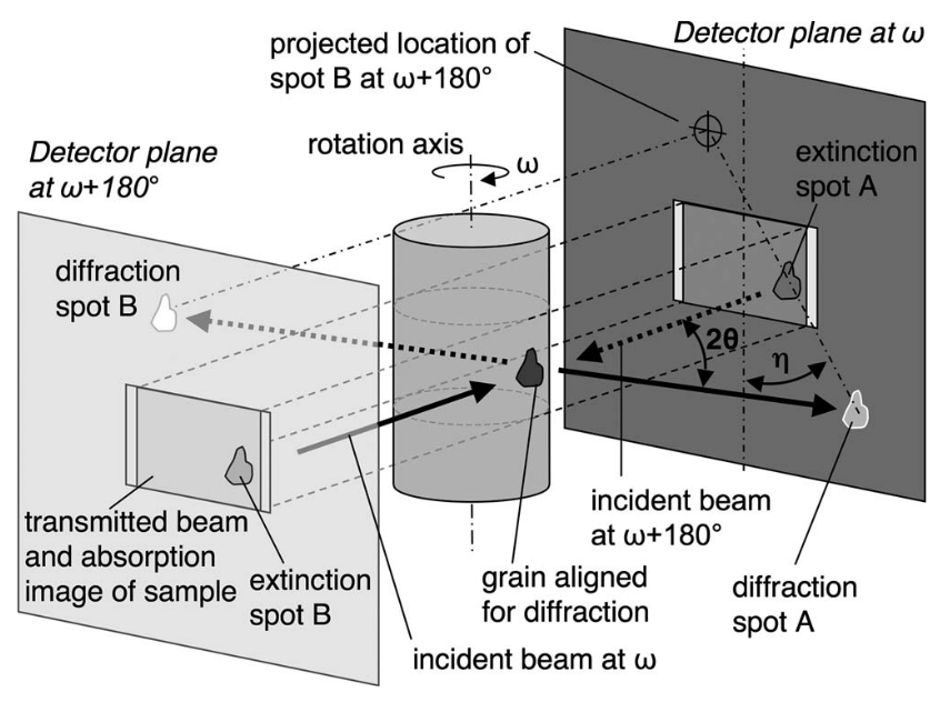
Fig. 36 Representation of a Friedel pair in the reference fixed to the sample.
Diffraction spot A appears at sample angle \(\omega\) . Its pair, spot B, is shown on the opposite
imaginary detector plane at angle \(\omega + \pi\). The diffraction path connecting both
passes through the grain of origin. From Ludwig RSI 2009 DOI#
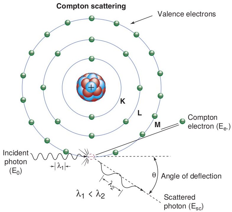
Compton scattering, inelastic and incoherent, is the dominant interaction for most
share of materials in a wide range of energy. The photon transfers a part
of its energy to the atom which expels a peripheral electron (therefore weakly bound).
total cross section \(\sigma_C\left/\rho\right. \approx \) cstt then \(\propto 1\left/E\right.\)
independent of \(Z\)
atom is ionized
loosely bound electron
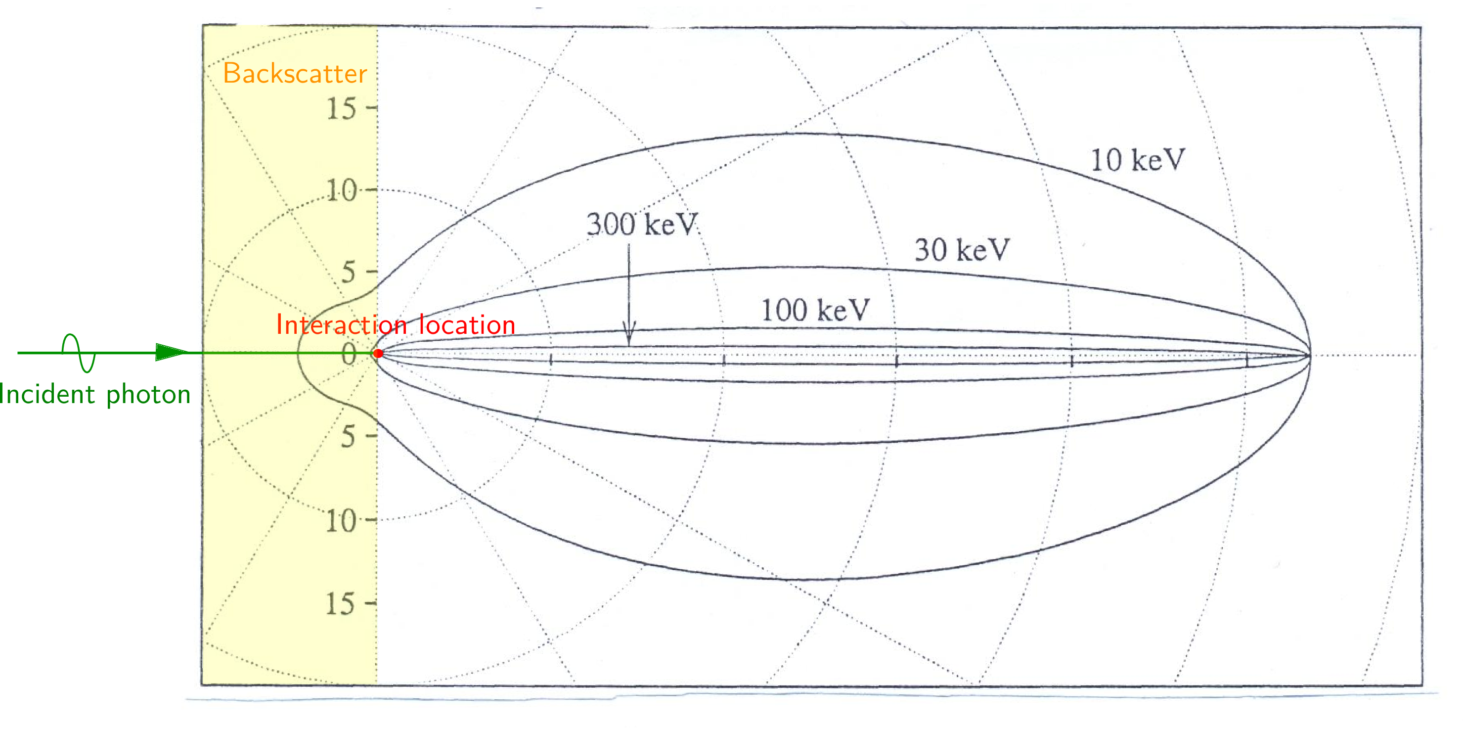
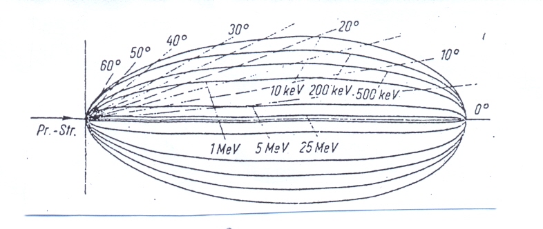
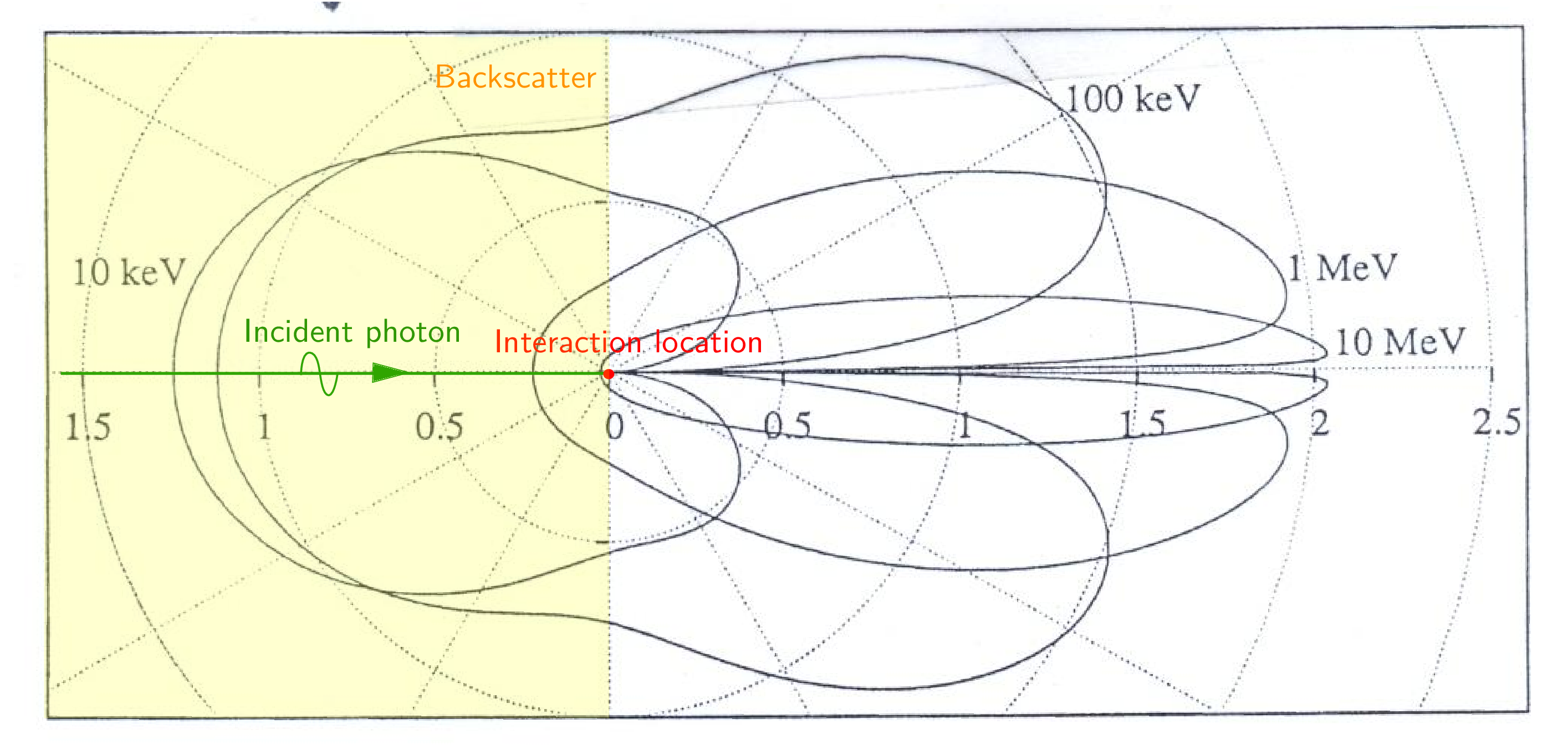
The angular differential cross section (DCS) is much more isotropic than for the Rayleigh
scattering: at low energy, the most likely direction for the scattered photon Compton is even backwards,
ie \(\theta \approx \pi\).
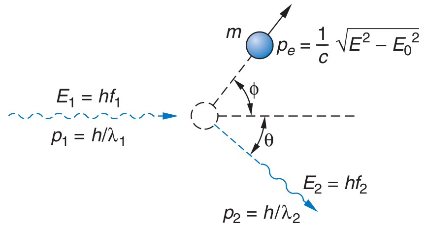
The laws of conservation of energy and momentum allow to model the energy of the scattered Compton
\(E_2\) photon as a function of the scattering angle \(\theta\). This law is decreasing monotonically
with \(\theta\), and the energy is maximum and close to the energy incident for small angles.
Energy-momentum relations (with \(E_0 = m_e c^2\) and \(p = |\boldsymbol{p}|\)): \(E_i^2 = (p_ic)^2\) with \(i\in\{1,2\}\) and \(E_e^2 = E_0^2 + (p_ec)^2\)
Conservation of the momentum (vector): \(\boldsymbol{p_1} = \boldsymbol{p_2} + \boldsymbol{p_e}\)
Conservation of the energy: \(E_1 + E_0 = E_2 + \sqrt{E_0 + (p_ec)^2}\)
This relationship assumes that the expelled Compton electron is at rest, in practice there is
Doppler broadening. The atom is therefore ionized as a result of this interaction, this is what gave
the terminology of “ionizing”.
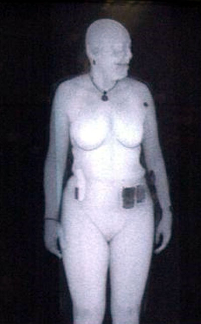
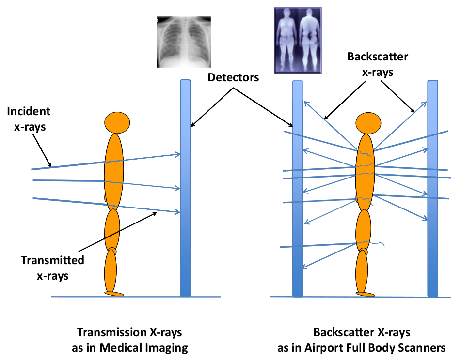
Compton backscattering has been the subject of scanning imaging protocol development.
whole body, especially for border control at airports. Source
collimated in a brush sweeps and turns around the person, the detector is the same
side as the source.
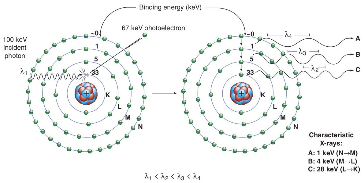
The photoelectric effect is a total absorption interaction, the photon transfers any its energy to
the atom. A strongly bound electron is expelled from the atom. This electron called photoelectron
leaves with a kinetic energy equal to that of the photon incident minus its initial binding
energy.
total cross section \(\tau\left/\rho\right. \propto Z^n\left/E^3\right.\) with \(n\in[3\;4]\)
shell discontinuitites
ionized atom
tightly bound electron
\(KE_{\mathrm{Photo-e}^{-}} = E - E_{\mathrm{binding}}\)
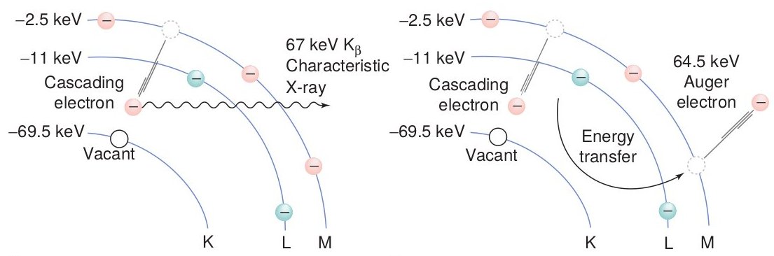
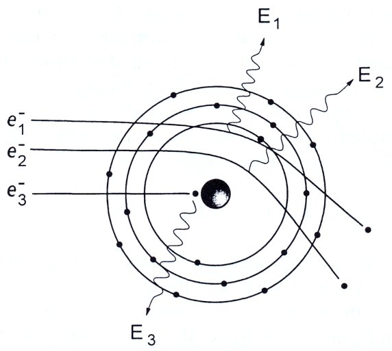
At this point the atom is ionized on an internal shell, a cascade of re-arrangement of the
electronic procession takes place and the associated energy releases result from a competition
between two phenomena exclusive: the expulsion of another but peripheral electron called the Auger
electron, or well the emission of a so-called fluorescence photon. The energies of fluorescent
radiation are characteristic of the atom (eg use to measure lead in paintings). See the NIST
database for the list of
transition energies per element and the XDB table for
the compiled list of emission lines. The photoelectric absorption depends also on the local
molecular structure: this phenomenon is used in the x-ray absorption spectroscopy (XAS).
Fig. 44 Atomic Relaxation (I atom example):* Fluorescence radiation (left) vs Auger electron (right)#
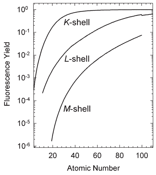
Fig. 45 Fluorescence yields for K, L, and M shells.#
The fluorescence efficiency is very close to 100% for materials with large atomic number. On the
other hand, for materials with low atomic number, there will be no fluorescence radiation but emission of
Auger electrons.
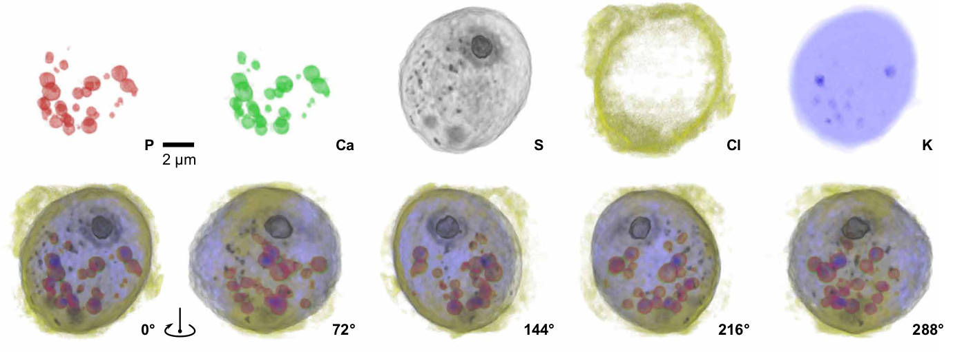
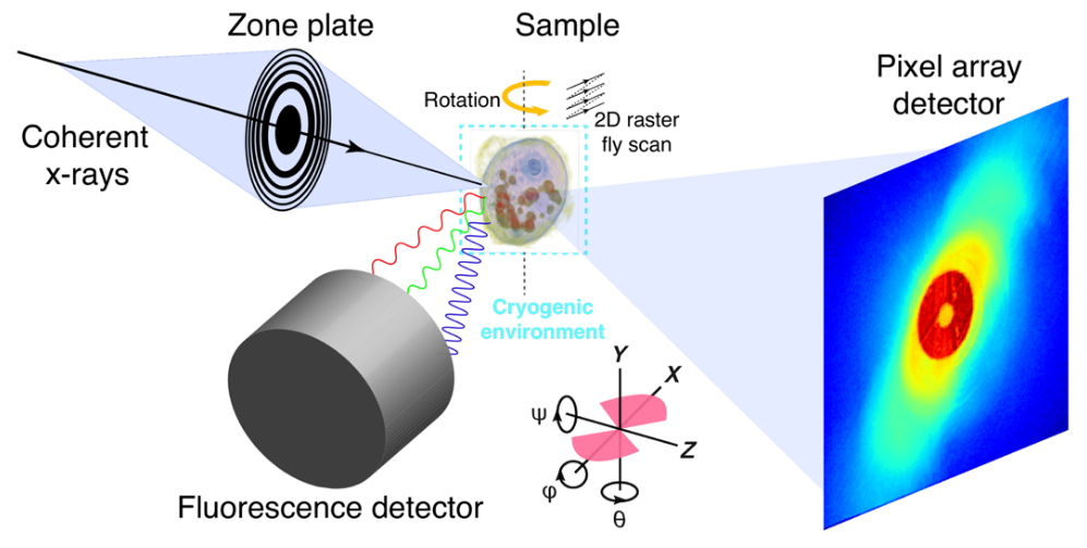
Fig. 46 Monochromatic 5.5 keV x-ray beam – Frozen-hydrated green algae cell. Top: different channels for the 0° projected view. Bottom: projected views. From Deng SA 2018 DOI#
Application to 3D fluorescence imaging of the different constituents of a cell.
Fig. 47 Experimental schematics for simultaneous x-ray flurescence and diffraction measurement. From Deng SA 2018 DOI#
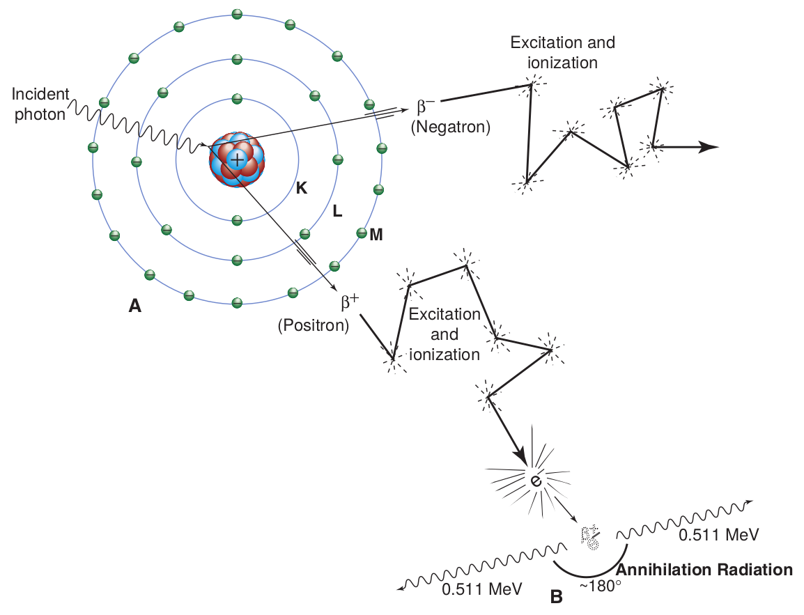
The pair production is a total absorption interaction, the photon transfers any its energy to the
atom. A pair of electron and its antiparticle, a positron, is created in the vicinity of the
atom. The remaning energy, ie the energy of the incident photon minus twice the rest mass of the
electron (ie 1.022 MeV), is transfered as kinetic energy to teh electron and positron.
Fig. 48 A high-energy incident photon is converted to an electron-positron pair (A). Both
the positron and the electron expend their kinetic energy by excitation and ionization in the matter they
traverse. However, when the positron comes to rest, it combines with an electron producing the two 511
keV annihilation-radiation photons (B). From The essential of physics of medical imaging.#
Characteristics:
dominant for high energy
total cross section proportional to atomic number
exists only for incident photon energies \(E>2m_ec^2=1.022\) MeV$
\(KE_{e^-} + KE_{e^+} = E - 2 m_{e}c^2\)
When the positron comes at rest, it is annihilated with a neighboring electron and two \(511\) keV are emitted in opposite directions. This electron-positron annihilation is the principle of PET medical imaging.
Photonuclear interaction (aka nuclear photoelectric effect) is the absorption of gamma-ray photons by atomic nuclei and the accompanying ejection of protons p, neutrons n, or heavier particles from the nuclei. The photonuclear cross-section has the appearance of a high energy resonance (eg around 14MeV for tungsten or 23MeV for carbon), with a distribution shape similar to a Lorentz function. The peak energy of the distribution of this giant dipole resonance (gdr) is directly related to the atomic mass,
and the full-width half maximum of the gdr distribution is small, around 7MeV. Nuclear fluorescence resonance (NRF) may also occur, it is a \((\gamma,\gamma')\) nuclear reaction. NRF is the process by which an excited nuclear state emits \(\gamma\)-rays of specific energies to de-excite to its ground state. NRF spectroscopy has been used in NDT to prevent illicit drug smuggling across borders and seaports (see Nature DOI).
Fig. 49 Photonuclear reactions triggered by a thunderstorm (see Nature DOI)#
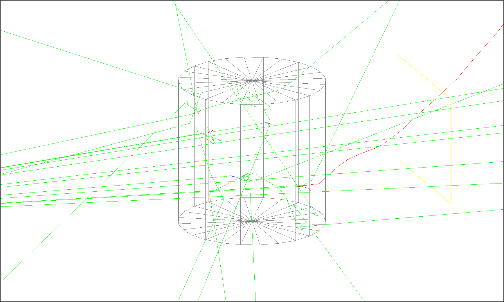
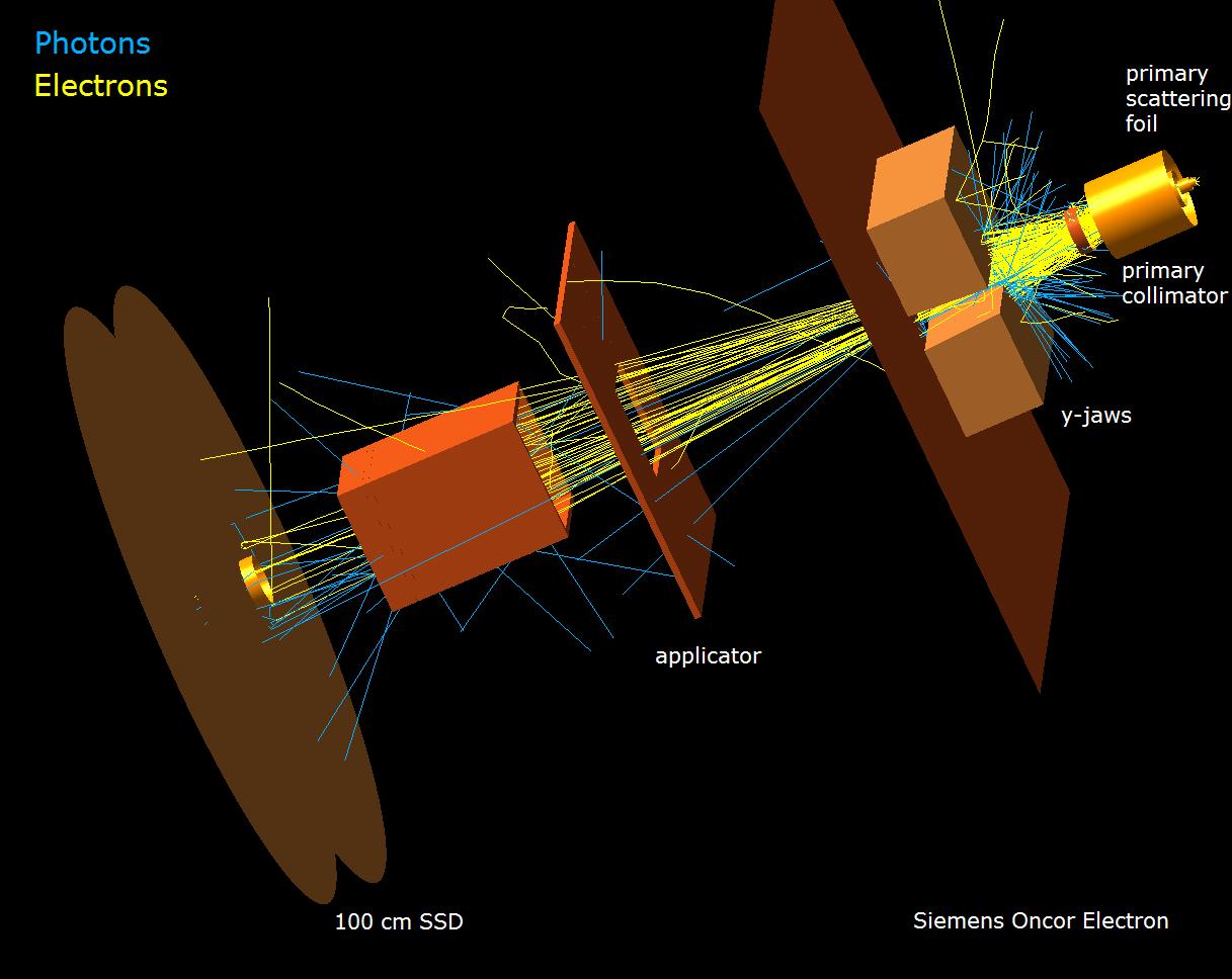
Fig. 50 12 MeV x-ray beam – Water cylinder (40cm diam.) in air – Photons in green (incident from the left), electrons in red, positrons in blue, and the detector in yellow on the right.#
X-ray imaging, which aims at detecting directly transmitted radiation only (ie without interaction), can be parasitized by the presence of many types of secondary radiation (Rayleigh and Compton scattering, Fluorescence…) as Fig. 50 shows. Electrons (and possibly positrons if the energy is greater than 1.02 MeV) are also by-products of interactions.
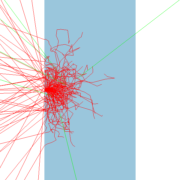
Fig. 51 100 electrons at 500 keV impinging on a W target (100 micron thick)#
Fig. 51 shows the traces (in red) of electrons of 500 keV impacting from the left a
W plate (100 microns thick and in vacuum). We see that the electrons have trajectories very
disturbed and travel less than 100 microns. On the other hand, on the hundred electron launched, a
few generated photons (in green).
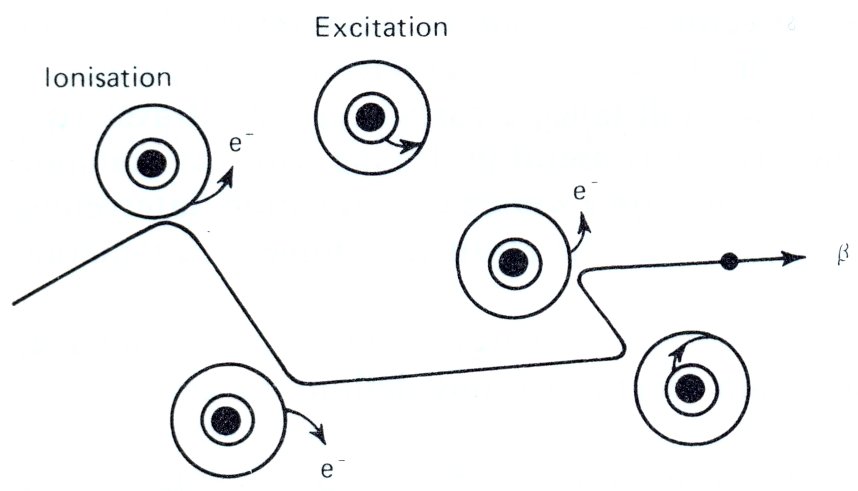
Electron-matter interactions are shared between collision (ionizations or excitation) and radiative processes. Collisions are more likely for electrons with low kinetic energies and might ionized atoms, therefore Fluorescence radiation may result from collisions. Radiative processes are more likely for electrons with very high kinetic energies and generate Bremsstrahlung x-ray photons.
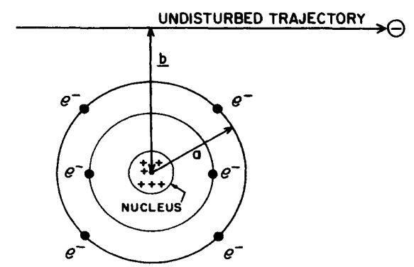
Fig. 52 Parameters in charged-particle collision with atoms: \(a\) is the classical
atomic radius; \(b\) is the classical impact parameter. From Attix DOI#
if \(b\approx a \Rightarrow\) hard collisions leading to excitation and ionisation, thus possibly emission of Auger electron or Fluorescence radiation)
if \(b \ll a \Rightarrow\) Coulomb-Force interactions with the external nuclear field, during which the electron is deflected in this process and gives a significant fraction of its kinetic energy to a photon (called Bresmstrahlung). From Attix DOI
radiative stopping power \(S_{\text{radiative}} \propto E_0^{-2} \Rightarrow\) negligible for heavy charged particles
secondary x-ray radiation: Fluorescence + Bremsstrahlung (see section X-ray production)
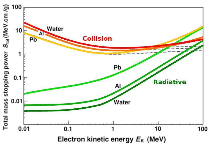
Fig. 55 Electron stopping powers for different materials#
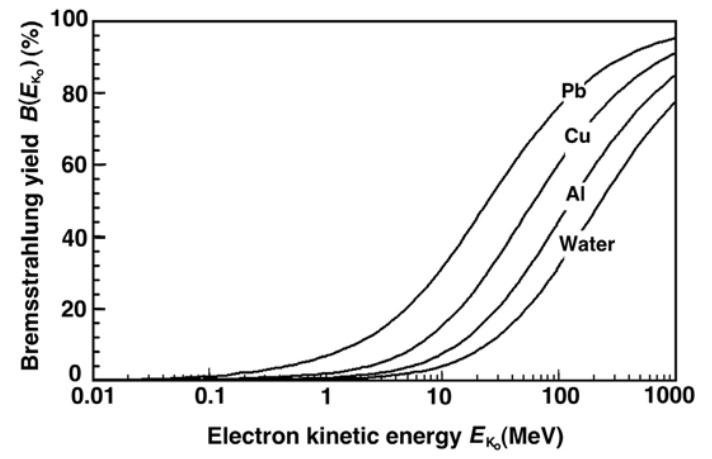
The radiative efficiency is very low (less than % as shown by
Fig. 56) in the range energy used in imaging. However, it is mainly Bremsstrahlung and less those of fluorescence (from ionizations by electrons) which are used in
x-ray generators to produce the radiation. The Heavy metal anodes increase radiative efficiency.
Bremsstrahlung radiation yield involved in the radiative fraction \(g\) (average radiative yield for all \(e^-\) produced) for defining the mass energy-absorption coefficient \(\mu_{en}\) (see section Linear energy-absorption coefficient)
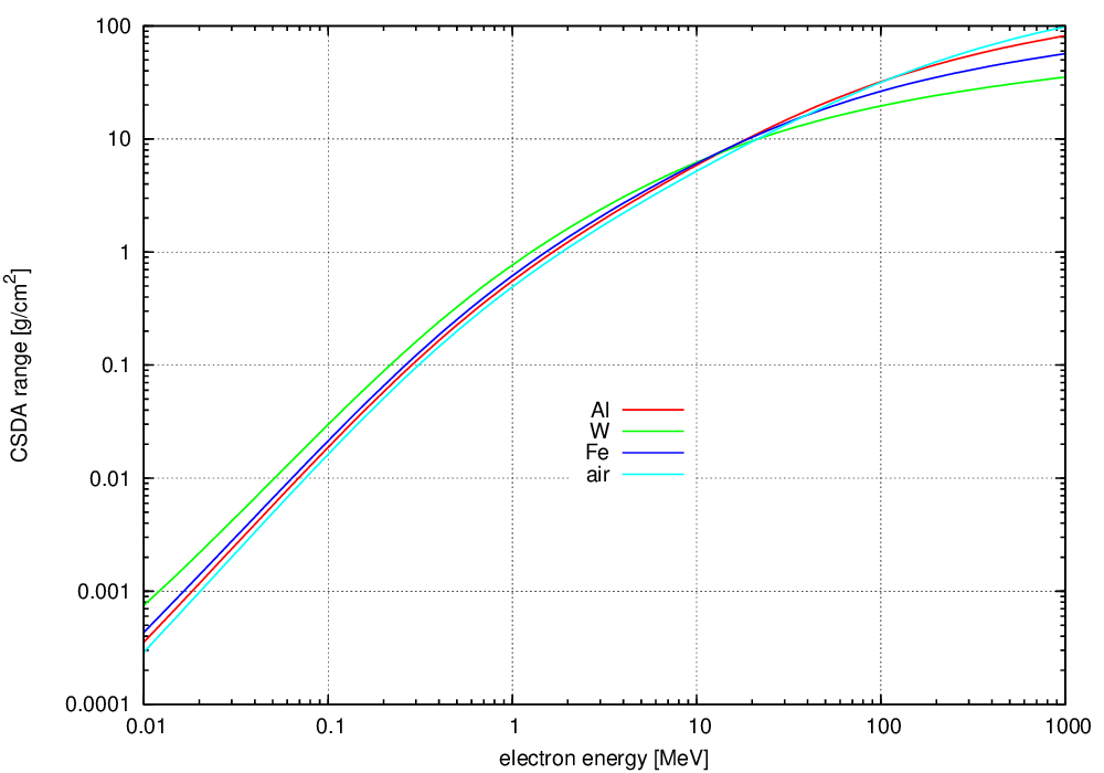
For a given kinetic energy of the electron, the maximum traversed range is defined by the CSDA (continuous slowing-down approwimation) range. The path of electrons, normalized in density, depends on the energy of the electrons but very
bit of the material. The electrons expelled during photon-matter interactions are absorbed locally (this is the notion of dose): the path of 100 keV electrons in water is
less than 200 microns.
Fig. 57 Continuous Slowing-Down Approwimation of (CSDA) the electron range#
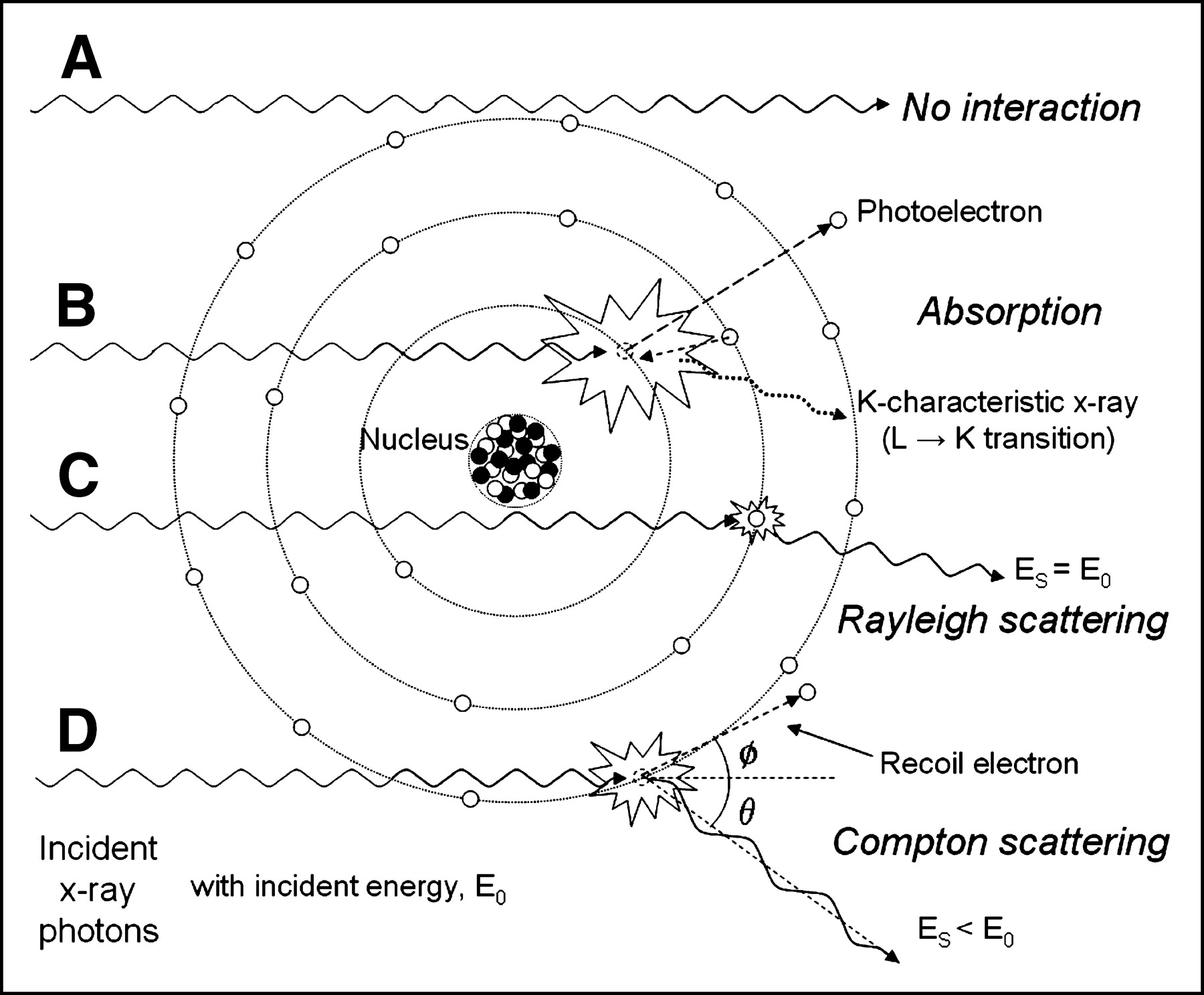
Fig. 58 Illustrative summary of x-ray and γ-ray interactions. (A) Primary, unattenuated beam does not interact with material. (B) Photoelectric absorption results in total removal of incident x-ray photon with energy greater than binding energy of electron in its shell, with excess energy distributed to kinetic energy of photoelectron. (C) Rayleigh scattering is interaction with electron (or whole atom) in which no energy is exchanged and incident x-ray energy equals scattered x-ray energy with small angular change in direction. (D) Compton scattering interactions occur with essentially unbound electrons, with transfer of energy shared between recoil electron and scattered photon, with energy exchange described by Klein–Nishina formula. From Seibert 2005; J Nucl Med Technol (33) pp.3–18#
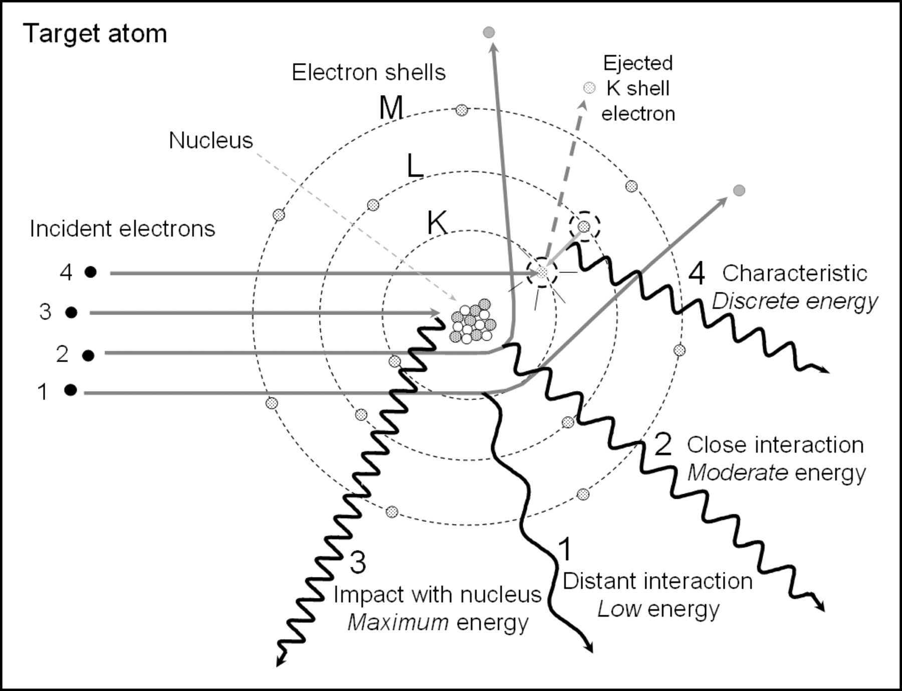
Fig. 59 X-ray production by energy conversion. Events 1, 2, and 3 depict incident electrons interacting in the vicinity of the target nucleus, resulting in bremsstrahlung production caused by the deceleration and change of momentum, with the emission of a continuous energy spectrum of x-ray photons. Event 4 demonstrates characteristic radiation emission, where an incident electron with energy greater than the K-shell binding energy collides with and ejects the inner electron creating an unstable vacancy. An outer shell electron transitions to the inner shell and emits an x-ray with energy equal to the difference in binding energies of the outer electron shell and K shell that are “characteristic” of tungsten. From Seibert 2004; J Nucl Med Technol (32) pp.139–147#
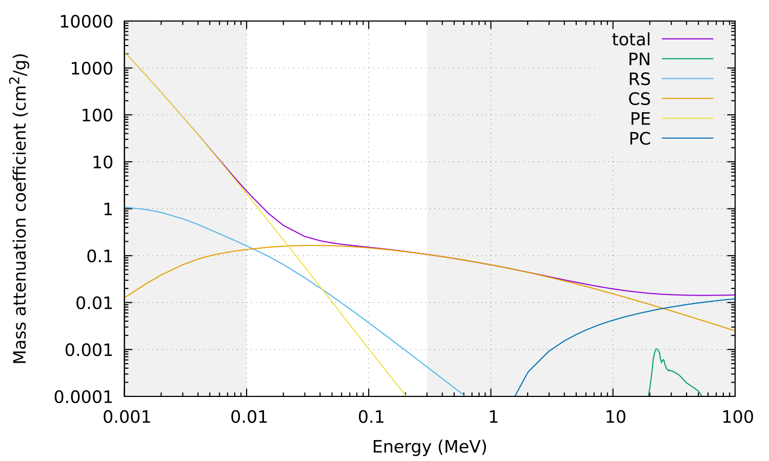
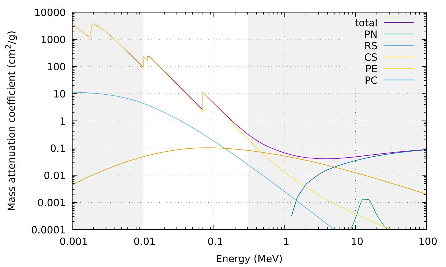
Mass attenuation coefficient curves for carbon (Fig. 60) and tungsten (Fig. 61). The
discontinuities for the photoelectric effect (PhE) are visible for tungsten because the electron
binding energies of the atom are greater (70 keV for the K layer of tungsten while it is only 0.3
keV for carbon).
Fig. 60 Mass attenuation coefficient \(\mu/\rho\) (in cm\(^2\cdot\)g\(^{-1}\)) of carbon (C)#
Fig. 61 Mass attenuation coefficient \(\mu/\rho\) (in cm\(^2\cdot\)g\(^{-1}\)) of tungsten (W)#
Note the relative constant of the coefficient of mass Compton scattering
attenuation (CS) between the two materials, while that of the photoelectric effect is much more
dominant for tungsten. The creation of electron-positron pair (PC) is a total absorption interaction
that occurs at very high energy.
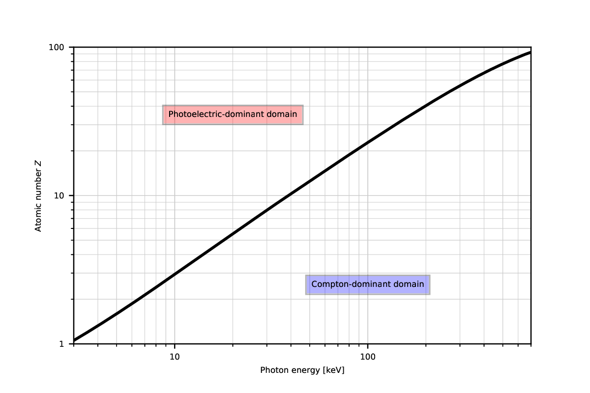
The iso-probability curve between the interactions by photoelectric effect and by scattering
Compton is shown in Fig. 62.
Materials with a low atomic number will essentially interact with
X-rays by Compton scattering, while heavy metals mainly by
photoelectric effect. These domains are usefull for the choice of energy (to minimize secondary radiations) or material (for radioprotection}
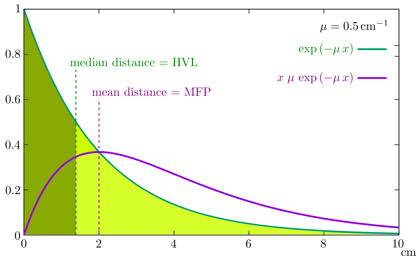
In radioprotection, two quantities based on the linear attenuation coefficient are usually used: the half-attenuation layer (or HVL) and the mean free path (or MFP). Figure Fig. 63 illustrates those two quantities for the case \(\mu=0.5\)cm\(^{-1}\).
Fig. 63 Illustration of half-attenuation layer (or HVL) and mean free path (or MFP)#
The half-attenuation layer or HVL (couche de demie-atténuation ou CDA) represents the thickness necessary to attenuate by a factor of 2
the number of photons transmitted without interaction.
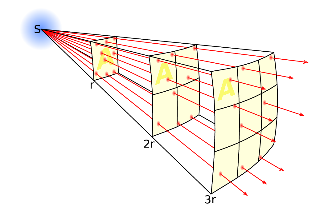
The divergence of the beam is directly conditioned by the solid angle between a surface
and the source of radiation. This relation can be approximated by an inverse relation-
is proportional to the square of the distance from the radiation source, considering
that the surface is small and perpendicular to the direction of propagation.
Diverging beam (no attenuation): Distance law
\[ N_1 d_1^2 = N_2 d_2^2 \]
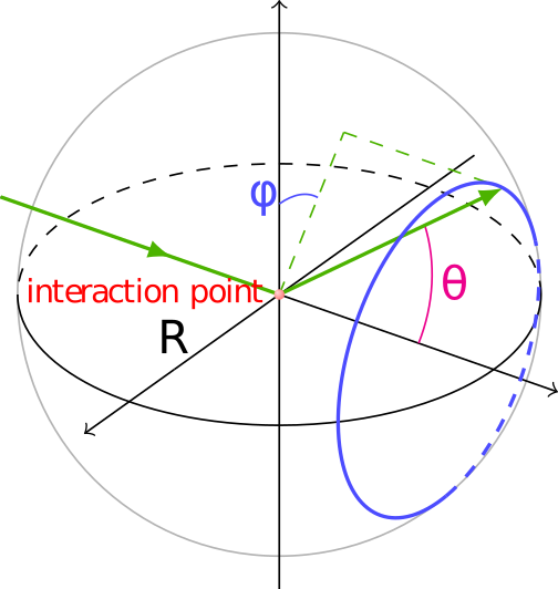
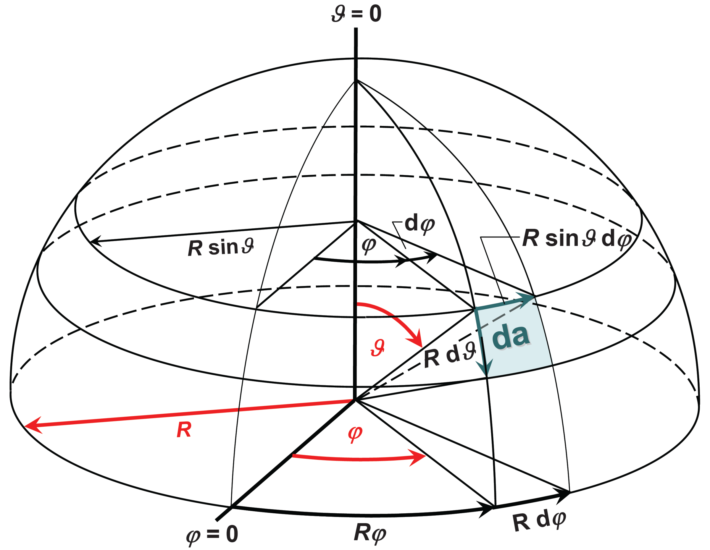
Solid angles should be used to be more precise if the x-ray source emission is expressed per solid angle (eg in \(4\pi\) for the whole space). To compute the number of photons passing through a given surface, we need to determine its solid angle, ie the equivalent spherical surface \(\text{d}a\) on a given sphere of radius \(R\).
NB : to account for secondary radiations, a build-up factor \(>1\) is sometimes used, especially in radioprotection to get a better estimate of all the radiations that pass through.
Wave phenomena are really present for X-rays, but the differences in indices being very small, it is
difficult to observe them with standard x-ray sources. But for a coherent x-ray beam, diffraction patterns
are much more likely to be visible.
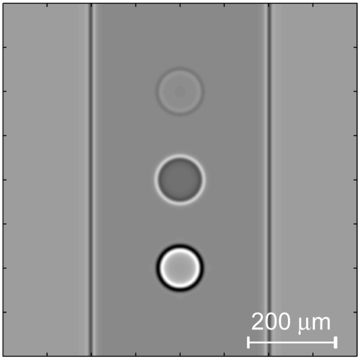
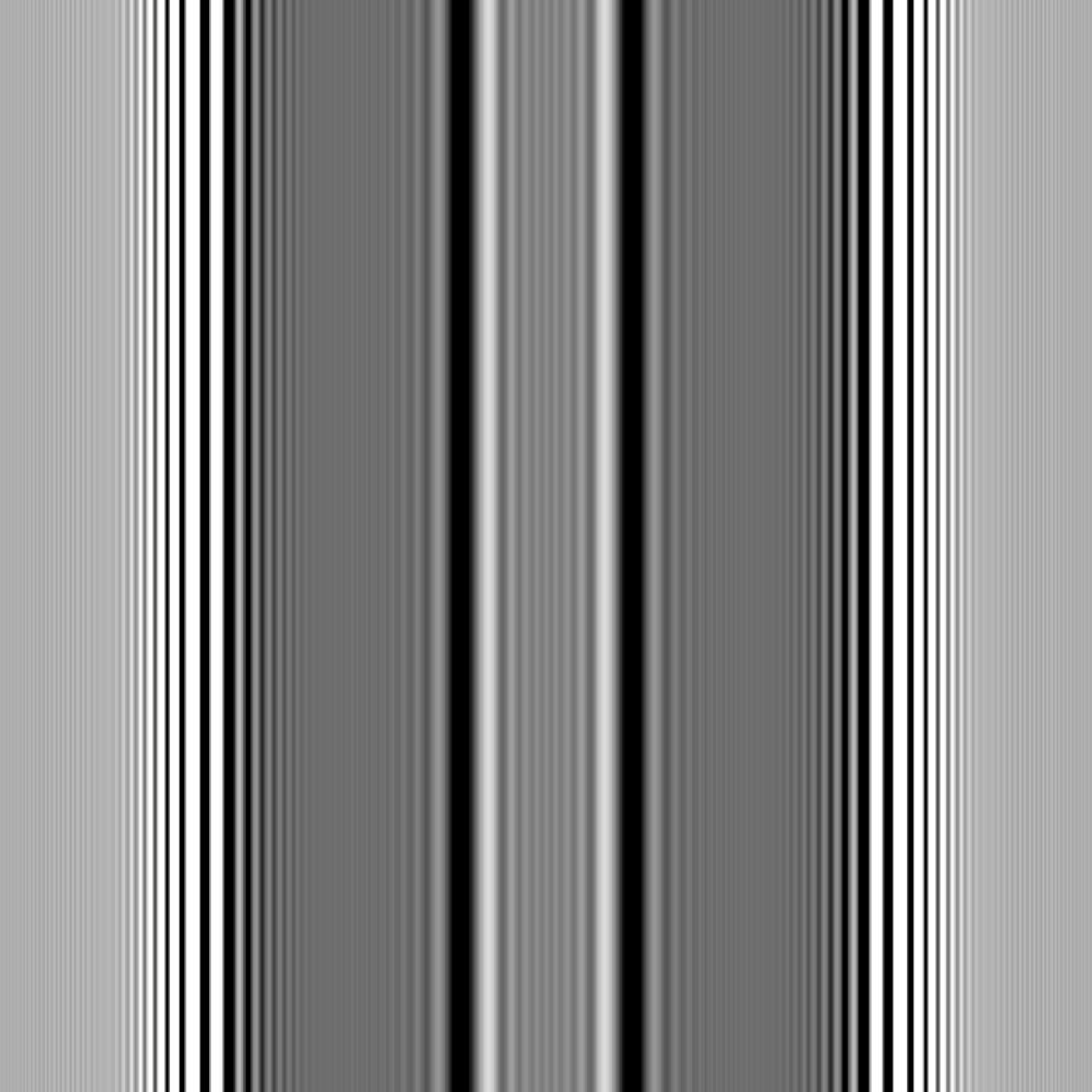
Fig. 66 Simulated noise-free phase-contrast image of an object consisting of a square rod of PMMA containing 100 microns spheres of water (upper), teflon (middle), and air (lower). DOI#
A link between the Beer-Lambert attenuation law and the propagation of the electromagnetic wave can
be established under some assumptions. Energy directly transmitted \(N_ {DT} E\) is therefore the
squared modulus of the wave, and the integral along the radius of the attenuation coefficient linear
\(\mu\) becomes the integral along the radius of the refractive index \(n\), of which the imaginary part
\(\beta\) is linked to \(\mu\). The exponential law is found so similar on the phase term with \(\delta\).
\[ u_0 = I_0 \exp \left( i \frac{2\pi}{\lambda} \int_{r \in ray} n(r) dr \right) \]
with
refraction index \(n(r) = 1 - \delta(r) + i \beta(r)\)
\(\delta(r) \propto \rho(r) \lambda^2\)
\(\beta(r) = \lambda \mu(r) (4 \pi)^{-1}\)
\[ u_0 = I_0 \exp \left( -\frac{2\pi}{\lambda} \beta T \right) \exp \left( - i \omega \left(t - \frac{T}{c}\right) \right) \exp \left( -i \frac{2\pi}{\lambda} \delta T \right) \]
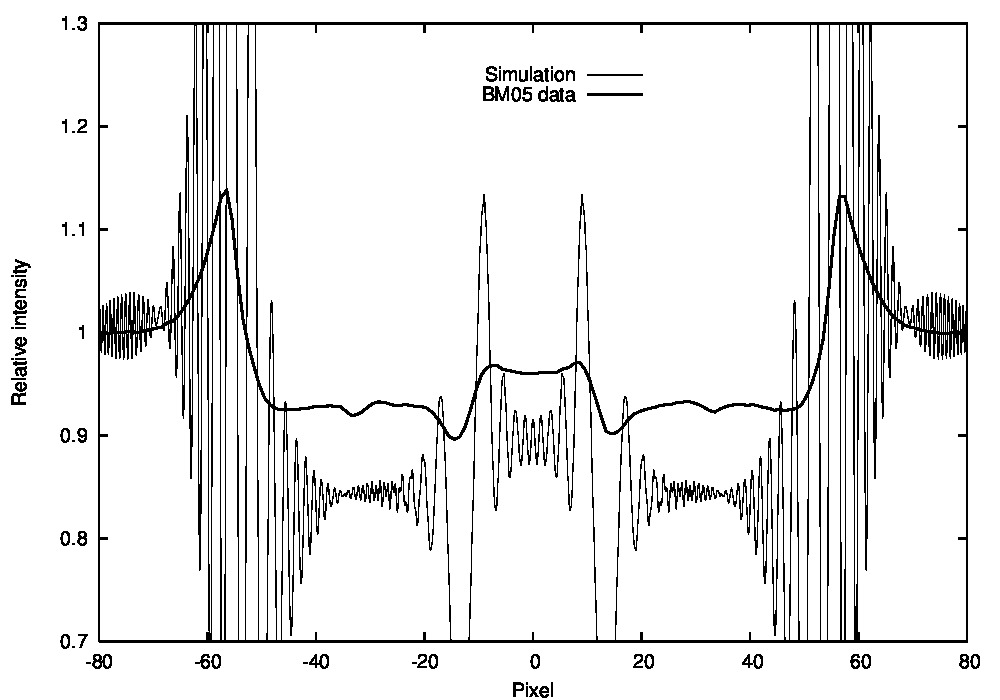
As an example, Fig. 68 to Fig. 72 illustrate Fresnel interference by a fiber 150 microns in diameter with a detector
placed at 56.7 cm from the fiber. We can clearly see the phase contrast on the acquired image. The
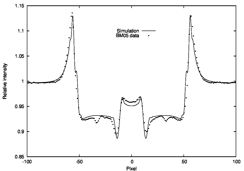
simulation reproduces this phenomenon well when the impulse response of the detector or PSF is
taken into account. These interferences have a very small spatial extent (a few microns).
Fig. 71 Profile across the fiber comparing the data with the simulation of the Fresnel x-ray diffraction#
Fig. 72 Idem Fig. 71 with the impulse response of the detector taken into account in the simulation#
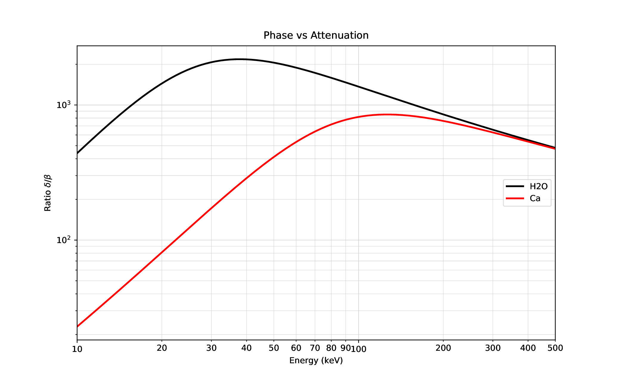
The interest in phase imaging is the gain in sensitivity. The phase of the wave is up to 1000 times
more sensitive to variations in density than its amplitude (see Fig. 73).
Fig. 73 Ratio of the phase component \(\delta\) over the attenuation component \(\beta\) in terms if the x-ray energy#
Fig. 81 Example of the Geant4-DNA Monte Carlo code#
In NDT to visualize the different secondary radiation contributions:
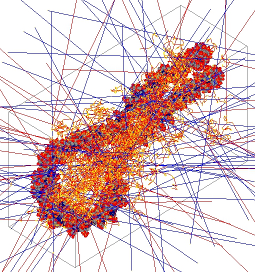
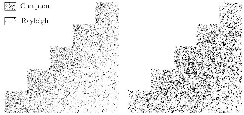
Fig. 82 Orthographic projection of the scattering events obtained with 100.000 incident photons. Left First-order scattering events. Right: higher order scattering. DOI#
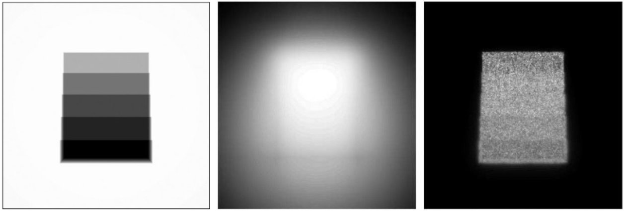
Fig. 83 Simulation of the 2D image of photon scattering behind a step wedge on a detector placed close to the wedge. Left: directly transmitted photons. Middle: first-order Compton scattered photons. Right: first-order Rayleigh scattered photons. DOI#
For further details
\(\mu/\rho\)database\(\Longrightarrow\) See XCOM from the National Institute of Standards and Technology (NIST)
Interactive plots of \(\mu\), the DCS \(\Longrightarrow\)Jupyter Notebook.
Monte Carlo simulations software \(\Longrightarrow\) See for example the Geant4 website of CERN