SIMRI: Interactive
interface
The figure given below presents the main window of this interface. The left upper part of the window presents the r, T1 and T2 profiles of the virtual object along the 1D direction. On this example, the object is composed of four different homogeneous parts. This profile can be interactively defined by the user. The user is also able to define a main field inhomogeneity profile associated to the object. The object definition can be saved on disk and reloaded. Note that up to two isochromats can be defined for an object corresponding to the water and fat protons.
The bottom part of the window concerns the sequence type and parameters that can be modified interactively, impacting the 1D MRI signal. The signal is displayed in the right upper part of the window. User can choose to display the RF signal through its module, phase, real and imaginary part. The reconstructed signal can be displayed as a signal and as a grey level line as it could appear in a complete 2D or 3D acquisition. On the example below, the image line is displayed as well as the magnitude of the RF signal and the reconstructed signal.
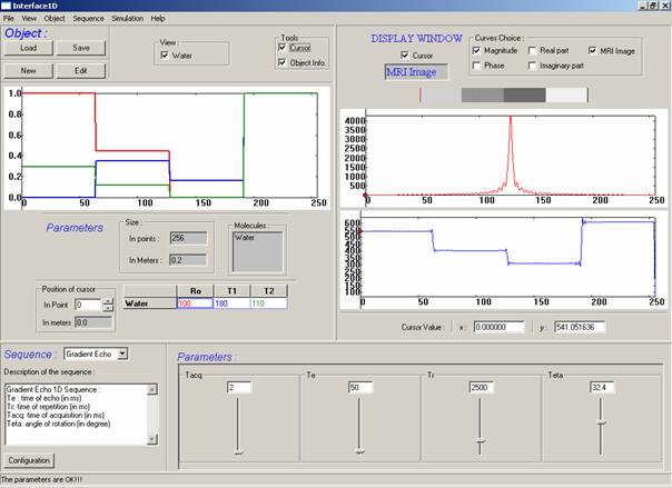
Object ro, T1, T2 profile (top left). Sequence choice and parameters (bottom). Signal display (top right) showing the module of the RF signal, the reconstructed signal and the corresponding image line.
Illustration
of the SpinPlayer interface
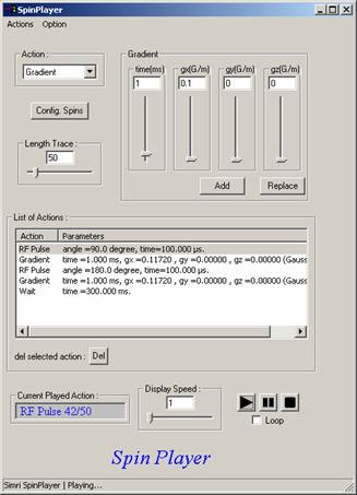
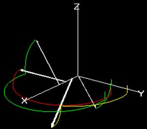
From the View menu of the main window, the user can call a second type of interface that we called the "SpinPlayer" and which is illustrated below. The main idea of the SpinPlayer is to offer a 3D visualization of the object spin magnetization vectors within the rotating frame during a sequence. Such visualization is presented c) with four spin magnetization vectors represented by the arrows.
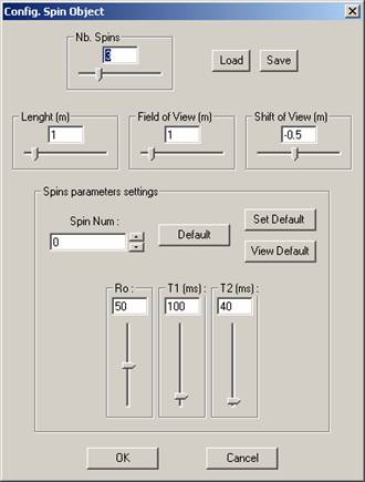
The user can configure (b) the number of spin magnetization vectors to view and their characteristics (r, T1, T2). He can also save or load different vector sets. The user can design a sequence by chaining events like RF pulse, gradient and precession (a). User sequence definition can be save and/or load.
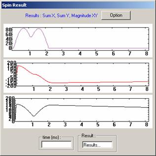
Once a sequence and a spin magnetization vector set are defined, the user chooses the display speed and the trace length of the spin vectors and then plays the sequence. During the play, the user observes the vector motions (Figure 24-c) and also the RF signals that would be acquired by two coils placed on the x and y axis as well as the magnitude of the combined complex signal (d). Note that the user can interact (zoom, rotation, translation) with the 3D spin vector visualization window during the play.
|
|
|
|
a) Sequence definition. |
b) Spin magnetization vector configuration. |
|
|
|
|
c) 3D view of the
spin magnetization vectors. |
d) Signal detected by orthogonal coils placed in the x-y plane. |