Context

Whereas the organ or tissue to be observed is usually a 3D scene, ultrasound systems provide most of the time only a 2D slice of the investigated media. Different approaches to extend ultrasound to 3D are possible. One very promising approach is to extend the principle of phased arrays to matrix arrays able to steer the ultrasound beam in 3D. One of the main limitations is that a fully sampled matrix array would typically count several thousands of elements whereas current scanners can drive only 128 to max 256 elements. The motivation of this work is to optimise 2D probe layouts of a fixed number of elements (N_el = 256) to perform 3D US imaging aiming at the same quality of 2D imaging.

Method

It is known that reducing the elements number by removing them on a regular basis leads to important grating lobe in the array directivity pattern. Such artifacts can be reduced by introducing randomness in the elements positionning. We propose to optimize the array elements layout using simulated annealing algorithms.

We have made several contributions in the optimization methods including the introduction of non grid positionning of DIAR-12c DIAR-13aDIAR-14 the elements and variable size DIAR-13b.

We have also proposed a realistic ultrasound model based on FIELD II (JA Jensen, DTU) to calculate the Energy function used in the optimization procedure ROUX-14 .

The Energy function U(S_n) is based on the radiated pattern RP_Sn( of the probe at state S_n.

To compute the radiated pattern thousands of pressure measurement points (PMPs) are located on the half-sphere of radius R_hs, where R_hs = focal distance (FIG. 1). They measure the pressure field (PF_Sn) which is transformed into RP_Sn by storing the maximum along time dimension, normalization and log compression as written in 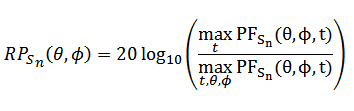Eq. 1:

Eq. 1

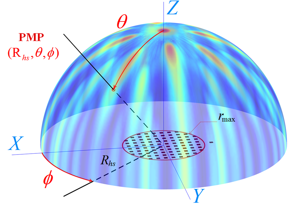
FIG 1 : Around 11.000 pressure measurement points (PMPs) are located on the half-sphere of radius R_hs centered on the probe S_n

The Energy function of the probe configuration U(S_n) is defined by 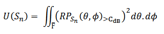Eq.2 :

Eq.2

We integrate the squared values of the RP_Sn above the maximum GLL and SLL constraint C_dB. The integration is not done on all the PMPs because the ones inside the main-lobe region (F) are excluded. The main-lobe region is defined as the points which are closer than (resolution/2) from the focal point.

Such a definiition drives the solutions to the main goals which are the resolution [< 1mm @ -6dB] and the side lobe level  [ C_dB = -30dB (in Tx or Rx - one way)].

Experiment

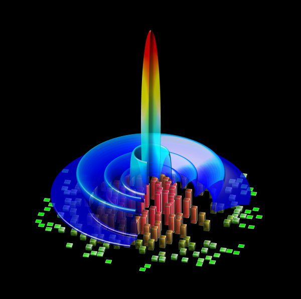
To illustrate the method we take a N_el = 256 elements probe with central frequency f_c = 7 MHz. Each element is a 200 µm square and the layout is limited inside a 55 λ aperture (r_{max =} 6 mm with c = 1540 m/s). The transmitted signal is a 3 sine-cycles (Hamming windowed) and we focalize at 25 mm on z-axis. At each iteration of the simulated algorithm, all the elements are single-wise translated of random values in [-100 µm; + 100 µm] in both lateral and elevation direction (overlapping situations are logically avoided) . The cost function is computed after each single perturbation which leads to over N_el x N_iterations = 256 x 10 000 = 2.560.000 simulations in our case:

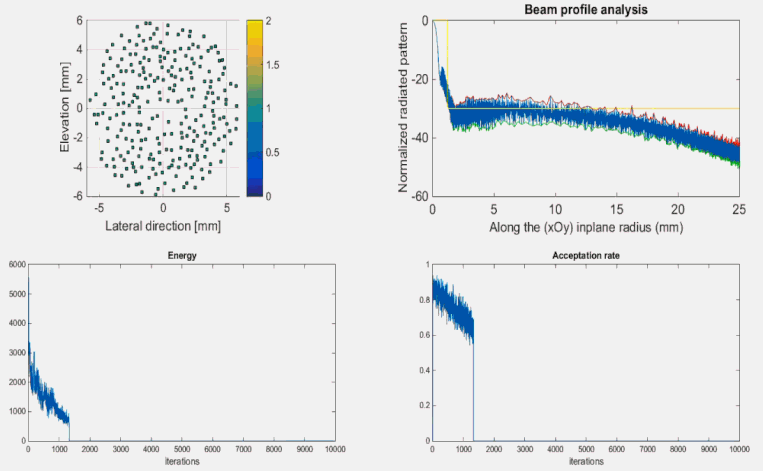
FIG 2 : The optimization process evolution.
The top-left graph shows the evolution of elements positions on the layout.

Both resolution (< 0.8 mm @ -6dB) and side-lobe level (< -30dB ) constraints were reached at the end of the optimization process.